E. D. Nering-linear Algebra And Matrix Theory-wiley (1976).pdf 3nw3a

m, then v(a) =n - p(a) � n - m > 0, so that a cannot be a monomorphism. Any linear transformation from a vector space into a vector space of higher dimension must fail to be an epimorphism. Any linear transformation from a vector space into a vector space of lower dimension must fail to be a monomorphism. Theorem 1.8. Let U and V have the same finite dimension n. A linear transformation a ofU into Vis an isomorphism if and only if it is an epimorphism. a is an isomorphism if and only if it is a monomorphism. PROOF. It is part of the definition of an isomorphism that it is both an epimorphism and a monomorphism. Suppose a is an epimorphism. p(a) = n and v ( a) = 0 by Theorem 1.6. Hence, a is a monomorphism. Conversely if a is a monomorphism, then v(a) = 0 and, by Theorem 1.6, p(a) =n. Hence, a is an epimorphism. D

J

1

Linear Transformations

33

Thus a linear transformation <1 of U into V is an isomorphism if two of the following three conditions are satisfied: ( 1) dim U =dim V, (2) <J is an epimorphism, (3) <J is a monomorphism. Theorem 1.9. p(r) = p('ra) + dim {lm(a) n K(r)}. PROOF. Let r' be a new linear transformation defined on Im(a) mapping Im(a) into W so that for all rJ. E Im(a), r1(rJ.) =r(rJ.). Then K(r') = Im(a) n K(r) and p(r') =dim r[lm(a)] =dim r<J(U) =p(r
takes the form p(r') + v(r') =dim Im(a), or p(ra) +dim {lm(a)

n

K(r)} = p(a).

D

Corollary 1.10. p(ra) =dim {Im(a) + K(r)} - v(r). PROOF. This follows from Theorem 1.9 by application of Theorem 4.8

of Chapter

I. D

Corollary 1.11.

If K(r)

c

Im(a), then p(a) = p(r
D

Theorem 1.12. The rank of a product of linear transformations is less than or equal to the rank of either factor: p(ra) =:;; min { p(r), p(a)}. PROOF. The rank ofr<J is the dimension ofr[a(U)] c r(V). Thus consider ing dim a(U) as the "n" and dim r(V) as the "m" of Theorem 1.3 we see that dim ra(U) p(r
Theorem 1.13. If <1 is an epimorphism, then p(ra) p(r). If r is a mono morphism, then p(ra) =p(a). �OF. If <J is an epimorphism, then K(r) c Im(a) = V and Corollary 1.ll applies. Thus p(ra) = p(a) - v(r) =m - v(r) = p(r). If r is a monomorphism, then K(r) = {O} c Im(a) and Corollary 1. ll applies. p(a). D p(a) - v(r) Thus p(ra) =

=

=

Corollary 1.14. The rank of a linear transformation is not changed by multiplication by an isomorphism (on either side). D Theorem 1.15. <1 is an epimorphism if and only if r<J 0 implies r =0. is a monomorphism if and only if r<J =0 implies <1 0. PROOF. Suppose <J is an epimorphism. Assume r<J is defined and r<J =0. If r =;C 0, there is a f3 E V such that r(/3) =;C 0. Since <J is an epimorphism, there is an rJ. EU such that r and r(f3i) 0 for =

T

=

=

=

=

34

Linear Transformations and Matrices

i :5: r. Then 7'<1

=

I

II

0 and 7' "# 0. This is a contradiction and, hence, a is an

epimorphism. Now, assume 7'<1 is defined and 7'<1 = 0. Suppose 7' is a monomorphism. If <1 "# 0, there is an ex EU such that a(cx) "# 0. Since 7' is a monomorphism, 7'<1(cx) "# 0. This is a contradiction and, hence, a 0. Now assume 7'<1 = 0 implies a = 0. If 7' is not a monomorphism there is an ex EU such that ex "# 0 and T(ot) = 0. Let {cx1' ... , ocn} be any basis of U. Define a(oci) = ex for each i. Then 7'<1(oci) = T(ot) = 0 for all i and 7'<1 0. This is a contradiction and, hence, 7' is a monomorphism. o =

=

7'1

Corollary 1.16. a is an epimorphism if and only if -r1<1 = 7'2<1 implies 7'2• 7' is a monomorphism if and only if 7'<11 7'<12 implies a1 = a2• =

=

The statement that

7'1<1 7'<11

=

and the statement that

7'2<1 implies 7'1 7'<12 implies <11

7'2 is called a right-cancellation, a2 is called a left-cancellat ;pn. transformation that can be cancelled ofi the =

=

Thus, an epimorphism is a linear

=

right, and a monomorphism is a linear transformation that can be cancelled on the left.

Theorem 1.17. Let A {oti. . . . , cxn} be any basis of U. Let B {/JI> ... , /Jn} be any n vectors in V ( not necessarily linearly independent). There exists a uniquely determined linear transformation a of U into V such that a(oci) pi =

=

=

for i

=

1,

2, . . . , n.

Since A is a basis of U, any vector

PROOF.

in the form

ix =

ex

EU can be expressed uniquely

L7=1 aicxi. If a is to be linear we must have a(cx)

=

n L aia(ot); i=l

=

n .L a;(3i EU. i=l

It is a simple matter to that the mapping so defined is linear. o

Corollary 1.18. Let C = {yi. . . . , Yr} be any linearly independent set in U, where U is finite dimensional. Let D = {o1, ... , or} be any r vectors in V. There exists a linear transformation a of U into V such that a(yi) = oi for i I, .. . , r. PROOF. Extend C to a basis of U. Define a(yi) = o; for i 1, . . . , r, =

=

and define the values of

a on

the other elements of the basis arbitrarily. This

will yield a linear transformation It should be clear that, if define

a.

a

with the desired properties. o

C is not already a basis, there are many ways to C is crucial

It is worth pointing out that the independence of the set

to proving the existence of the linear transformation with the desired prop erties. Otherwise, a linear relation among the elements of a

C would impose

corresponding linear relation among the elements of D, which would mean

that D could not be arbitrary.

1

I

35

Linear Transformations

Theorem 1.17 establishes, for one thing, that linear transformations really do exist. Moreover, they exist in abundance. The real utility of this theorem and its corollary is that it enables us to establish the existence of a linear transformation with some desirable property with great convenience.

All

we have to do is to define this function on an independent set.

Definition. A linear transformation 71' of V into itself with the property that 2 71' = 71' is called a projection. Theorem 1.19. If 71' is a projection of V into itself, then V = and 71' acts like the identity on Im('TT').

lm('TT') ffi

K('TT')

2

PROOF.

For ex E V, let ex1 ='TT'(ex). Then 'TT'(ex1)= 71' (ex)= 'TT'(ot) = ex1• This

shows that 71' acts like the identity on Im('TT'). Let cx2 = ex - ex1. Then 'TT'(ex2) =

'TT'(ex) - 'TT'(ex1) = ex1 - ex1= 0. Thus ex= ex1 + ex2 where ex1 E l m('TT') and ex2 E K('TT'). Clearly, Im('TT') n K('TT')= {O}. D T a

' I

I I

7r(a)

Fig. 1

If S = Im('TT') and T= K( 71' ), we say that 71' is a projection of V onto S along T. In the case where V is the real plane, Fig. l indicates the interpretation of these words. ex is projected onto a point of S in a direction parallel to T. EXERCISES 1. Show that a((x1, x2)) Let

2. a1a2

and

3.

Let

a1((x1, x2)) <1 2<11· U

where k <

4. that

=

(x2, x1)

defines a linear transformation of R2 into

/

itself.

Let

a

=

n.

V

=

=

(x2, -x1) and a2((xi. x2))

Rn

and

Describe

let

Im(a)

a((x1, x2, x3, x4))

=

a((x1, x2, K(a).

•

•

•

=

(x1, -x2).

, xn))

=

Determine

a1 + a2,

(x1, x2,..., xk> 0, .

.

. , O)

and

(3x1 - 2x2 - x3 - 4x4, x1 + x2 - 2x3 - 3x4). a.

Show

is a linear transformation. Determine the kernel of

5. Let a((x1, x2, x3))

=

(2x1 + x2 + 3x3, 3x1 - x2 + x3, -4x1 + 3x2 + x3).

Find

36

Linear Transformations and Matrices I II

a basis of

a(U).)

a(U). (Hint: Take K(a).

particular values of the

Find a basis of

x;

to find a spanning set for

6. Let D denote the operator of differentiation,

dy d2 y 2 D(y) _d , D (y) - D[D(y)] _ - d 2, etc. x x Show that Dn is a linear transformation, and also that p(D) is a linear transforma tion if p(D) is a polynomial in D with constant coefficients. (Here we must assume that the space of functions on which D is defined contains only functions differen tiable at least as often as the degree of p(D).) 7. Let

case

aT

U

=

and

V and let

Ta

always true that 8. Let

ex

=

U

=

a

and

be linear transformations of

T

are both defined.

GT

V

=

=

U

into itself. In this

Construct an example to show that it is not

Ta.

P, the space of polynomials in x with coefficients in R.

For

L�=o a;xi let n

a(ex)

L ia;xi-l

=

i=O

and

T(ex) Show that

aT

1, but that

=

n

=

Q·

L -.-'-

i=O I

+ 1

xi+l.

� 1.

TO"

9. Show that if two scalar transformations coincide on

U

then the defining

scalars are equal.

10.

Let

a

11.

{exi. . . ., exn} be a , a(exn)} are known, then the value

be a linear transformation of U into V and let A

basis of U. Show that if the values {a(ex1), of a(ex) can be computed for each ex EU.

.

.

•

Let U and V be vector spaces of dimensions n and

m,

=

respectively, over the

same field F. We have already commented that the set of all linear transformations of

U

into V forms a vector space.

Let A

=

Give the details of the proof of this assertion.

{ex1, . . . , exn} be a basis of U and B = {Pi. ..., Pm} be a basis of V.

be the linear transformation of

U into

V such that

( )

{o

G;; cxk

Show that

=

{a;; Ii= 1, . . . , m;j = 1, .

if

k � j,

p,.

1"f

k

. .

, n} is

12. Show that 1.6 to

13.

T defined

U

p(a) :::;: p(Ta) V'.)

into V and

+

on

Show that max

{O, p(a)

+

T

a;1

= j.

a basis of this vector space.

For the following sequence of problems Jet dim be a linear transformation of

Let

U=

n

and dim V

=

m.

Let

a

a linear transformation of V into W.

v(T). (Hint :

Let V'

p(T) - m} :::;: p(Ta)

=

a(U) and

:::;: min

apply Theorem

{p(T), p(a)}.

2

I

37

Matrices

14. Show that max m

{n

- m + v ( T) , v ( a) } � v ( Ta) � min

{n, v( a)

+ v ( T) } .

(For

= n this inequality is known as Sylvester's law of nullity.) 15. Show that if v ( T) =0,then p ( Ta) = p(a).

v(a) = 0 (Hint: Let m

16. It is not generally true that

example to illustrate this fact.

p(Ta)

implies

= p(T).

Construct an

be very large.)

17. Show that ifm =nandv(a) =0,then

p(Ta)

= p(T).

18. Show that if a1 and a2 are linear transformations of U into V, then

p(a1 19. Show that

+

a2) � min {m,n, p(a1)

lp(a1) - p(a2)1

p(a1

�

+

+

p(a2)}.

a2).

20. If S is any subspace of V there is a subspace T such that V = S EB T. Then

a; = a;1 + a;2 where a;1 E S and a; onto a;1 is a linear transformation.

every x E V can be represented uniquely in the form

a;2 E

T. Show that the mapping rr which maps

Show that T is the kernel of rr.

projection of V onto

Show that rr2

=

rr. The mapping rr is called a

S along T.

21. (Continuation) Let rr be a projection. Show that 1 What is the kernel of 1 that rr(l - rr)

=

-

-

rr is also a projection.

rr? Onto what subspace is 1 - rr a projection? Show

0.

2 I Matrices Definition.

A matrix over a field F is a rectangular array of scalars. The

array will be written in the form

(2.1)

whenever we wish to display all the elements in the array or show the form of the array.

A matrix with m rows and n columns is called an m x

n

matrix. An n x n matrix is said to be of order n. We often abbreviate a matrix written in the form above to

[a;;] where

the first index denotes the number of the row and the second index denotes

\

the number of he column.

The particular letter appearing in each index

position is immaterial; it is the position that is important.

With this con

a;; is a scalar and [a;;] is a matrix. Whereas the elements a;; and aki need not be equal, we consider the matrices [a;;] and [akiJ to be identical since both [a;;] and [ak1] stand for the entire matrix. As a further convenience we often use upper case Latin italic letters to denote matrices; A [a;1]. vention

=

Whenever we use lower case Latin italic letters to denote the scalars appearing


38

I II

in the matrix, we use the corresponding upper case Latin italic letter to denote the matrix. The matrix in which all scalars are zero is denoted by 0 (the third

The ai; appearing in the array [a;;] are called the elements of [a;;]. Two matrices are equal if and only if they have exactly the same elements. The main diagonal of the matrix [a;;] is the set ofelements , att} where t = min {m, n}. A diagonal matrix is a square matrix {a11, use of this symbol!).

•

.

•

in which the elements not in the main diagonal are zero. Matrices can be used to represent a variety of different mathematical con cepts. The way matrices are manipulated depends on the objects which they represent. Considering the wide variety of situations in whlcfimatrices have found application, there is a remarkable similarity in the operations performed on matrices in these situations. There are differences too, however, and to understand these differences we must understand the object represented and what information can be expected by manipulating with the matrices. We first investigate the properties of matrices as representations of linear trans formations. Not only do the matrices provide us with a convenient means of doing whatever computation is necessary with linear transformations, but the theory of vector spaces and linear transformations also proves to be a power

ful tool in developing the properties of matrices. Let U be a vector space of dimension n and V a vector space of dimension m, both over the same field F. Let A= {1X1, , 1Xn} be an arbitrary but fixed basis of U, and let B {{31, , f3m} be an arbitrary but fixed basis of V. Let <J be a linear transformation of U into V. Since <1(1X;) E V, <1(1X;)

=

•

•

•

•

•

•

can be expressed uniquely as a linear combination of the elements of B;

m a(IX;) = ! a;;f3;· i=l We define the matrix representing <J with respect to the bases A and the matrix A = [a;;].

(2.2) B to be

The correspondence between linear transformations and matrices is actually one-to-one and onto.

Given the linear transformation

= [a;;]

a,

the

a;;

exist because Bspans V, and they are unique because Bis linearly independent.

= !:'=1 a;;{J;

On the other hand, let A

<1(1X;)

for each

be any m x n matrix. We can define IX; EA, and then we can extend the proposed

linear transformation to all of U by the condition that it be linear. Thus, if� =

!7=1 X;IX;, we define

n a(�)= LX;<1(1X;) i=l

= j�/;c� a;;{J;) = i� (�1a;;X;) {J;..

(2.3)

2

I Matrices

39

a can be extended to all of U because A spans

U, and the result is well defined

(unique) because A is linearly independent. Here are some examples of linear transformations and the matrices which Consider the real plane R2

represent them.

(0, 1)}. A 90°

=

U

=

Let A= B = {(1, 0), (I, 0) onto (0, I) and 0 ( , 0) + 1 (0, and

V.

rotation counterclockwise would send

(0, 1) onto (- 1, 0). Since a ((l, 0)) a((O, 1)) = ( -1) (l, 0)+ 0 (0, I), a is represented

it would send

=

·

·

·

I

·

by the matrix

I)

[O -I] 1

0 .

The elements appearing in a column are the coordinates of each image of a basis vector under a transformation. In general, a rotation counterclockwise through an angle of () will send

(1, 0) onto

(cos(), sin()) and

(0, 1)

onto (-sin(), cos()), Thus this rotation

is represented by

[

cos()

-sin()

Suppose now that =

(2.4)

cos() .

sin()

by the matrix B

]

r is another linear transformation of U into V represented

[b;1]. Then for the sum a + r we have

(a+ r)(cx1)

=

m

m

i=l

i=l

a(cx1) + r(cx1) = L a;1{3; + L h;1/3; m

=

I (a;1+ b;1)f3;·

(2.5)

i=l

is represented by the matrix [aii + b;1]. Accordingly, we sum of two matrices to be that matrix obtained by the addition of the corresponding elements in the two arrays; A + B [aii + b;1] is

Thus

a+ r

define the

=

the matrix corresponding to

a+ r.

The sum of two matrices is defined if

and only if the two matrices have the same number of rows and the same number of columns. If

a is any scalar, for the linear transformation aa we have ( a a)(cx 1) =

m

m

i=l

i=l

(2.6)

a L a;1{3; = L (aa;1){3;.

[aa;1]. We therefore define scalar multiplication by the rule aA [aa;1]. Let W be a third vector space of dimension r over the field F, and let C {Yi. ... , Yr} be an arbitrary but fixed basis of W. If the linear trans formation a of U into V is represented by the m x n matrix A [a;1] and the Thus aa is represented by the matrix =

=

=

40


I II

linear transformation T of V into W is represented by the r x m matrix

B = [bk;],

what matrix represents the linear transformation T<1 of U into W? (T<1)(oc;) ='T(<1(oc;)) ='T

c� ) a;;,8;

m

=2 a;;T(,8;) i�l

i� Ct ) = t (�1 ) a;;

=

bkirk

bk;a;; Yk·

k

Thus, if we define ck1=.2�1 bk;a;1, then C the product transformation Ta. of Band

A,

in that order:

=

(2.7)

[ck1] is the matrix representing C the matrix product

Accordingly, we call

C= BA.

For computational purposes it is customary to write the arrays of B and

A

side by side.

The element ck; of the product is then obtained by

multiplying the corresponding elements of row k of B and column j of A and adding. We can trace the elements of row k of

B

with a finger of the

left hand while at the same time tracing the elements of column j of a finger of the right hand.

A with

At each step we compute the product of the

corresponding elements and accumulate the sum as we go along.

Using

this simple rule we can, with practice, become quite proficient, even to the point of doing "without hands." Check the process in the following examples: -1

-1

�J � � rl � �J =

-2

2

-

0

3

-2

-2 .

All definitions and properties we have established for linear transformations can be carried over immediately for matrices. For example, we have: 1. 0

·A =0.

(The "O" on the left is a scalar, the "O" on the right is a

matrix with the same number of rows and columns as

A.)

·A=A. 3. A(B + C)=AB + AC. 4. (A+ B)C=AC+ BC. 5. A(BC)= (A,B)C. 2. 1

Of course, in each of the above statements we must assume the operations proposed are well defined.

For example, in

3,

Band

C

must be the same

2

I

41

Matrices

size and A must have the same number of columns as B and C have rows. The rank and nullity of a matrix A are the rank and nullity of the associated linear transformation, respectively.

Theorem 2.1. is equal to n.

For an m x n matrix A, the rank of A plus the nullity of A

The rank of a product BA is less than or equal to the rank of

.either factor. These statements have been established for linear transformations and therefore hold for their corresponding matrices. D The rank of <1 is the dimension of the subspace Im( a) of V. Since Im( a) is spanned by

{a(cx.1),

•

•

,

•

a(cx.n)}, p(a)

is the number of elements in a

{a(cx.1), , a(cx.n)}. Expressed a(cx.1) = !:,1 ai1{3i is represented by the m-tuple (a11 a2 1, , a m1), which is the m-tuple in column j of the matrix [ai1]. Thus p(a) = p(A) is also equal to the maximum number of linearly inde

maximal linearly independent subset of

.

•

•

in of coordinates, ,

•

•

•

pendent columns of A. This is usually called the column rank of a matrix A, and the maximum number of linearly independent rows of A is called

the row rank of A.

We, however, show before long that the number of

linearly independent rows in a matrix is equal to the number of linearly independent columns.

Until that time we consider "rank" and "column

rank" as synonymous.

(2.3),

Returning to Equation

(x1,

•

•

•

, xn)

we see that, if � E U is represented by

and the linear transformation <1 of U into V is represented

by the matrix A =

[ai1],

aa) E Vis represented by (y1, n (i = 1, . . . , m). Yi= 1Lai1X1 �1 then

•

•

•

,

Ym)

where

(2.8)

In view of the definition of matrix multiplication given by Equation we can interpret Equations

where

Y=

(2.8)

[": ]

Y=AX

and

X=

["]

This single matric equation contains them equations in We have al;eaay used the n-tuple .

(2.9)

Xn

Ym

� = L��i xi cx.i

(2.7)

as a matrix product of the form

(x1,

•

•

•

,

xn)

•

(2.8).

to represent the vector

Because of the usefulness of equation

(2.9)

convenient to represent � by the one-column matrix X.

we also find it

In fact, since it is


42

somewhat wasteful of space and otherwise awkward to display one-column matrices we use the n-tuple

(x1,

.

.

, xn) to represent not only the vector � [x1 xn] is a one-row

•

but also the column matrix X. With this convention matrix and

(x1,

•

•

•

•

•

•

, xn) is a one-column matrix.

Notice that we have now used matrices for two different purposes, (1) to represent linear transformations, and matric equation Y

=

(2) to represent vectors. The___single

AX contains some matrices used in each wa y.

EXERCISES

1.

J [ : -:1 [ : [-: -1[ 1 n :] [�] [ �:]. [ _:

the matrix multiplication in the following examples:

[:

(a)

-

2

_

:

6

-

0

=

(c)

9 7

-2

]

11 4 .

-

2

_

(b)

_

6

1

3

0

-2

-1

,

=

15 4

.

�

2

2. Compute 9

[:

7

_

-,�t:J

Interpret the answer to this problem in of the computations in Exercise

[� : : :] [-:

3. Find AB and BA if

A

=

B

0

4. Let

a

1 0

1

'

=

-5

_

: : :]

-6

=

_

_

-7

-8 .

be a linear transformation of R2 into itself that maps

(0, 1) onto ( -1, 2). Determine the matrix representing B {(l, O), (0, 1)}. bases A

and

=

1.

a

(1, 0) onto (3, - 1 ) with respect to the

2

43

I Matrices 5. Let

a

be a linear transformation of

R2 into itself that maps (1, 1) onto (2, -3)

and

O. -1) onto (4, -7). Determine the matrix representing a with respect to the B { O. O), (0, 1)}. (Hint: We must determine the effect of a when it is applied to (1, O) and (0, 1). Use the fact that O. 0) to. 1) + to. -1) and the linearity of a. ) bases A

=

=

=

6. It happens that the linear transformation defined in Exercise

that is,

a

4 is one-to-one,

does not map two different vectors onto the same vector. Thus, there is

a linear transformation that maps

(3, -1) onto (1, 0) and (-1, 2) onto (0, 1).

This linear transformation reverses the mapping given by

a.

Determine the matrix

representing it with respect to the same bases.

7. Let us consider the geometric meaning of linear transformations. A linear R2 into itself leaves the origin fixed (why?) and maps straight

transformation of

lines into straight lines. (The word "into" is required here because the image of a straight line may be another straight line or it may be a single point.) Prove that the image of a straight line is a subset of a straight line.

(Hint:

Let

a

be represented

by the matrix

Then

a

maps

(x, y) onto (a11x + a12y, a21x + a22y). Now show that if (x, y) c its image satisfies the equation ax + by

satisfies the equation

=

(aa22 - ba21)x 8. (Continuation)

+

(a11b - a12a)y

=

(a11a22 - a12a21)c.)

We say that a straight line is mapped onto itself if every

point on the line is mapped onto a point on the line (but not all onto the same point) even though the points on the line may be moved around.

(a )

A linear transformation maps

(1, 0)

onto

(-1, O) and (0, 1) onto (0, -1).

Show that every line through the origin is mapped onto itself. Show that each such line is mapped onto itself with the sense of direction inverted. This linear transformation is called an

inversion

with respect to the origin. Find the matrix

representing this linear transformation with respect to the basis

(b)

A linear transformation maps

(1, 1)

onto

fixed. Show that every line perpendicular to the itself with the sense of direction inverted.

x1

+

x2

=

(-1, -1) line x1 + x2

{0, 0), (0, 1)}.

and leaves (1, -1) 0 is mapped onto

=

Show that every point on the line

0 is left fixed. Which lines through the origin are mapped onto them

selves? This linear transformation is called a

reflection about the line x1

+

x2

=

0.

Find the matrix representing this linear transformation with respect to the basis

{(1, O), (0, 1)}. Find the matrix representing this linear transformation with respect to the basis {(1, 1), (1, -1)}. (c)

A liner transformation maps

(1, 1)

onto

(2, 2) and 0, -1) onto (3, -3). (1, 1) and

Show that the lines through the origin and ing through the points

(1, -1)

are mapped onto themselves and that no other lines are mapped onto

thems�ves. Find the matrices representing this linear transformation with respect to the bases

{(1, 0), (0, 1)}

and

{(1, 1), (1, -1)}.


44

(d) A linear transformation leaves (1, 0) fixed and maps (0, 1) onto (1, 1). Show

c is mapped onto itself and translated within itse� distance that each line x2 equal to c. This linear transformation is calJed a shear. Which lines through the =

origin are mapped onto themselves?

Find the matrix representing this linear

transformation with respect to the basis

{(1, O), (0, 1)}.

A linear transformation maps (1, 0) onto (/3, � D and (0, 1) onto ( - �;, 153). Show that every line through the origin is rotated counterclockwise through the

(e)

angle ()

=

arc cos

/3.

This linear transformation is calJed a

rotation.

Find the

matrix representing this linear transformation with respect to the basis

(0, 1)}.

{(1, 0),

(f) A linear transformation maps (1, 0) onto (t, t) and (0, 1) onto (t, t). Show 3c is mapped onto the single point (c, c). that each point on the line 2x1 + x2 The line x1 - x2 0 is left fixed. The only other line through the origin which is mapped into itself is the line 2x1 + x2 0. This linear transformation is calJed =

=

=

a projection onto the line x1 - x2

=

0 parallel to the line 2x1 + x2

=

0. Find the {(1, O),

matrices representing this linear transformation with respect to the bases

(0, 1)} and {(1, 1), (1,

-

2) }

.

9. (Continuation) Describe the geometric effect of each of the linear transforma 2 tions of R into itself represented by the matrices

(a)

(d)

(Hint:

[: �] [� :]

[: :J [� :J

(b)

(e)

(c)

(f)

[� �] [! -:] 5

5

•

In Exercise 7 we have shown that straight lines are mapped into straight

lines. We already know that linear transformations map the origin onto the origin. Thus it is relatively easy to determine what happens to straight lines ing through the origin. For example, to see what happens to the x1-axis it is sufficient to see what happens to the point

(1, O).

Among the transformations given appear a

rotation, a reflection, two projections, and one shear.)

10. (Continuation) For the linear transformations given in Exercise 9 find all lines through the origin which are mapped onto or into themselves. 2 R3 and a be a linear transformation of U into V that 11. Let U R and V =

maps

(1, 1)

represents

a

(0, O, 1)} in 12. What

=

1, 0). Determine the matrix that {(1, O), (0, 1)} in B {(1, 0, 0), (0, 1, O), (1, 0).) R3• (Hint: !(1, 1) - H-1, 1) is the effect of multiplying an n x n matrix A by an n x n diagonal

onto (0,

1,

2) and

( -1, 1)

with respect to the bases A

onto (2,

=

=

=

matrix D? What is the difference between AD and DA?

13.

Let

such that

a

and b be two numbers such that

a

'¥ b.

Find all 2

x

2 matrices A

45

I Non-singular Matrices

3

14. Show that the matrix C = [a;b;] has rank one if not all ai and not all b; are zero. (Hint: Use Theorem 1.12.) 15. Let a, b, e, and d be given numbers (real or complex) and consider the function f(x) =

ax+ b

ex+ d .

--

Letg be another function of the same form. Show thatg/whereg/(x) =g(/(x)) is a function that can also be written in the same form. Show that each of these functions can be represented by a matrix in such a way that the matrix representing gfis the product of the matrices representingg and/ Show that the inverse function exists if and only if ad - be 716 0. To what does the function reduce if ad

-

be = 0?

16. Consider complex numbers of the form x+ yi (where x and y are real numbers and i2 = -1) and represent such a complex number by the duple (x, y) in R2• Let a+ bi be a fixed complex number. Consider the function f defined by the rule f (x+ yi) = (a + bi)(x+ yi) = u+ vi.

(a) Show that this function is a linear transformation of R2 into itself mapping (x, y) onto (u, v). (b) Find the matrix representing this linear transformation with respect to the basis { (1, 0), (0, 1)}. (c) Find the matrix which represents the linear transformation obtained by using + di in place of a+ bi.

c

Compute the product of these two matrices. Do they

commute? (d) Determine the complex number which can be used in place of a+ bi to obtain a transformation represented by this matrix product. How is this complex number related to a+ bi and c+ di?

17. Show by example that it is possible for two matrices A and B to have the same rank while A2 and B2 have different ranks.

3 I Non-singular Matrices Let us consider the case where U

=

V, that is, we are considering trans

formations of V into itself.

Generally, a homomorphism of a set into itself

is called an endomorphism.

We consider a fixed basis in V and represent

the linear transformation of V into itself with respect to that basis. case the matrices are square or n x n matrices.

In this

Since the transformations

we are considering map V into itself any finite number of them can be iterated in any order.

The commutative law does not hold, however.

The same

remarks hold for square matrices. They can be multiplied in any order but

46


the commutative law does not hold.

I

II

For example

[: �] [: �] [: �], [: �] [: �] [: :1 =

=

The linear transformation that leaves every element of V fixed is the identity transformation. the scalar identity.

We denote the identity transformation by

1,

Clearly, the identity transformation is represented by

the matrix I= [c5i;] for any choice of the basis. Notice that IA= AI= A for any order

n

n.

x

n

matrix A.

I is called the

identity matrix,

or

unit matrix,

of

If we wish to point out the dimension of the space we write In for

the identity matrix of order by the matrix Definition.

al.

n.

The scalar transformation

Matrices of the form

a is represented al are called scalar matrices.

A one-to-one linear transformation

itself is called an

automorphism.

a of a vector space onto

An automorphism is only a special kind of

isomorphism for which the domain and codomain are the same space.

a, the mapping a-1(a)

If

ix. is called the inverse transformation of a. The rotations represented in Section 2 are examples of automorphisms. a(ix.)

=

Theorem 3.1.

The inverse

=

a-1

of an automorphism a is an automorphism.

Theorem 3.2 A linear transformation T of an n-dimensiona/ vector space into itself is an automorphism if and only if it is of rank n; that is, if and only if it is an epimorphism. Theorem 3.3. A linear transformation a of an n-dimensional vector space into itself is an automorphism if and only if its nullity is 0, that is, if and only if it is a monomorphism. PROOF (of Theorems

3.1, 3.2, and 3.3).

These properties have already

been established for isomorphisms. D Since it is clear that transformations of rank less than

n

do not have

inverses because they are not onto, we see that automorphisms are the only linear transformations which have inverses. that has an inverse is said to be said to be

singular.

non-singular

or

A linear transformation

invertible;

otherwise it is

Let A be the matrix representing the automorphism

a, and let A-1 be the matrix representing the inverse transformation a-1•

The matrix A-1A represents the transformation a-1a. identity transformation, we must have A-1A= I. transformation of a-1 so that aa-1 A-1 as the

=

1 and

Since a-1a is the

But a is also the inverse

AA-1= I.

We shall refer to

inverse of A. A matrix that has an inverse is said singular or invertible. Only a square matrix can have an inverse.

to be

non

3 I Non-singular Matrices

47

On the other hand suppose that for the matrix A there exists a matrix

B such that BA=I. therefore,

Since I is of rank n, A must also be of rank n and,

A represents an automorphism

a.

Furthermore,

the linear

transformation which B represents is necessarily the inverse transformation

a1 since the product with

a

must yield the identity transformation.

Thus

B= A-1• The same kind of argument shows that if C is a matrix such that AC=I, then C= A-1• Thus we have shown: Theorem 3.4. AB=I.

If A

If

A and B are square matrices such that BA=I, then

and B are square matrices such that AB=I, then BA = I.

In either case B is the unique inverse of A. D Theorem 3.5.

(2)

If A

(AB)-1 =B-1A-1,

and B are non-singular, then

(1)

aA is non-singular and (aA)-1=a-1A-1• In view of the remarks preceding Theorem

PROOF.

(3)

AB is non-singular and

A-1 is non-singular and (A-1)-1=A,

3.4

for a -:;t. 0,

it is sufficient in

each case to produce a matrix which will act as a left inverse.

(1) (2)

(3)

(B-1A-1)(AB)= B-1(A-1A)B=B-1IB=B-1B=I. AA-1=I. (a-1A-1)(aA)=(a-1a)(A-1A)=I. D

Theorem 3.6.

If A is non-singular, we can solve uniquely the equations

XA = B and AY=B for any matrix B of the proper size, but the two solutions

need not be equal. Solutions exist since (BA-1)A=B(A-1A)= B and A(A-1B)=

PROOF.

(AA-1)B

=

B. The solutions are unique since for any C having the property

that CA= B we have C=CAA-1= BA-1, and similarly with any solution of AY=B. D As an example illustrating the last statement of the theorem, let

A= Then

[� �], G -2] -3,

A-1=

X= BA-1 =

[� ]

and

-2 1

'

B=

G �]. [-3 -2] 2

Y=A-1B=

1 .

We add the remark that for non-singular A, the solution of XA =B exists and is unique if B has

n

without change.

3.6

columns, and the solution of AY= B exists

and i s unique if B has n rows.

The proof given for Theorem

applies

48

Linear Transformations and Matrices Theorem 3.7.

I

II

The rank of a (not necessarily square) matrix is not changed

by multiplication by a non-singular matrix. PROOF. 2.1

AB

Let

A

be non-singular and let

is of rank r s p, and

The proof that

BA

A-1(AB)

B

be of rank p. Then by Theorem

=Bis of rank p s r.

Thus r

=

p.

is of rank p is similar. o

Theorem 1.14 states the corresponding property for linear transformations. The existence or non-existence of the inverse of a square matrix depends on the matrix itself and not on whether it represents a linear transformation of a vector space into itself or a linear transformation of one vector space into another. Thus it is convenient and consistent to extend our usage of the term "non-singular" to include isomorphisms.

Accordingly any square

matrix with an inverse is non-singular. Let U and V be vector spaces of dimension n over the field F.

Let A

=

{ a.:i. ... , a.:n} be a basis of U and B {/31, , f3n} be a basis of V. If � 27=1 xirxi is any vector in U we can define a(�) to be 27=1 x;/3;. It is easily seen that a is an isomorphism and that � and a(�) are both repre n sented by (x1, , xn) E f . Thus any two vector spaces of the same =

•

•

•

=

•

•

.

dimension over F are isomorphic.

As far as their internal structure is con

cerned they are indistinguishable.

Whatever properties may serve to dis

tinguish them are, by definition, not vector space properties. EXERCISES

[: :J

[=

1. Show that the inverse of 2

A�

3

4

A-1

is

0

0

3

�i[: _J

2. Find the square of the matrix A

-2

2

-2

-�]

1 .

-2

What is the inverse of A? (Geometrically, this matrix represents a 180° rotation about the line containing the vector (2, 1, 1).

The inverse obtained is therefore

not surprising.)

3. Compute the image of the vector (1, -2, 1) under the linear transformation represented by the matrix

A=

[: : :] 0

Show that A cannot have an inverse.

2 .

3 I

Non-singular Matrices

49

4. Since

[

we can find the inverse of

3

-

-5

1 2

]

by solving the equations

3x11 - 5x12 -Xll + 2X12

=1 =0 3X21 - 5X22 =0 -X21 + 2x22 = 1.

Solve these equations and check your answer by showing that this gives the inverse matrix. We have not as yet developed convenient and effective methods for obtaining the inverse of a given matrix.

Such methods are developed later in this chapter

and in the following chapter.

If we know the geometric meaning of the matrix,

however, it is often possible to obtain the inverse with very little work.

5.

The matrix

=arc cos -}.

8

[! -:J

represents a rotation about the origin through the angle

What rotation would be the inverse of this rotation? What matrix

would represent this inverse rotation? Show that this matrix is the inverse of the t

n

gi

:� :: ::� [ T

rix

O

-

-1

l

]

0

represents a reflection about the line

What operation is the inverse of this reflection?

x1

+

x2 =0.

What matrix represents the

inverse operation? Show that this matrix is the inverse of the given matrix. 7. The matrix

[� : ]

represents a shear. The inverse transformation is also a

shear. Which one? What matrix represents the inverse shear? matrix is the inverse of the given matrix. 8. Show that the transformation that maps

automorphism of

3 f.

(x1, x2, x3)

onto

Show that this

(x3, -xi. x2)

is an

Find the matrix representing this automorphism and its

inverse with respect to the basis

{(l, 0, O), (0, 1, O), (0, 0, 1)}.

9. Show that an automorphism of a vector space maps every subspace onto a

subspace of the same dimension.

10.

Find an example to show that there exist non-square matrices A and B

such that AB n

x m

n

x

=I.

Specifically, show that there is an

matrix B such that AB is the

m

n identity. Prove in general that if

identity matrices.

x m m

identity.

m

x

n matrix A and an

Show that BA is not the

;en, then AB and BA cannot both be

Linear Transfo rmations

50

and Matrices I

II

4 I Change of Basis

We have represented vectors and linear transformations as n-tuples and matrices with respect to arbitrary but fixed bases. A very natural question arises:

What changes occur in these representations if other choices for

bases are made?

The vectors and linear transformations have meaning

independent of any particular choice of bases, independent of any coordinate systems, but their representations are entirely dependent on the bases chosen. Let A =

Definition.

{or.i. ..., or.n}

and A'

=

{or.�, ..., or.�}

be bases of the

vector space U. In a typical "change of basis" situation the representations of various vectors and linear transformations are known in of the basis A, and we wish to determine their representations in of the basis A'.

In this connection, we refer to A as the "old" basis and to A' as

the "new" basis.

Each

or.;

is expressible as a linear combination of the

elements of A; that is,

n or.;= L P; ;or.i. = i l matrix P = [p;;] is called the matrix of transition

The associated

(4.1) from the

basis A to the basis A'. The columns of P are the n-tuples representing the new basis vectors in of the old basis.

This simple observation is worth ing as

it is usually the key to determining P when a change of basis is made. Since the columns of P are the representations of the basis A' they are linearly independent and P has rank Now let ;

L7=1 xior.i

=

n. Thus P is non-singular.

be an arbitrary vector of U and let ;

=

L�=l x;or.;

be the representation of ; in of the basis A'. Then

;tx;or.; =;tx; Ct Pi;or.;) =i� c� P;;X; ) or.; .

;=

(4.2)

Since the representation of ; with respect to the basis A is unique we see that

X;

= "i,j=1p;;x;.

Notice that the rows of P are used to express the

old coordinates of ; in of the new coordinates.

For emphasis and

contradistinction, we repeat that the columns of P are used to express the new basis vectors in of the old basis vectors. Let X=

(x1,

.

.

•

,

xn) and X'

=

(x�,

.

.

•

,

x�) be n

the vector ; with respect to the bases A and A'.

{x; = "i,j=1p;;x;}

x I matrices representing

Then the set of relations

can be written as the single matric equation

X=PX'.

(4.3)

4

I Change

of

51

Basis

Now suppose that we have a linear transformation a of U into V and that A = {a;;] is the matrix representing a with respect to the bases A in U and B = {f3i. ... , f3m} in V. We shall now determine the representation of a with respect to the bases A' and B.

m

(4.4)

=I i=l a;;{J;. Since B is a basis, a;; = I;=1 a;kh; and the matrix

A' = [a;11 representing a with respect to the bases A' and B is related to A by the matric equation

(4.5)

A' =AP.

This relation can also be demonstrated in a slightly different way. For an arbitrary $ =I�1 x;rx1 EU let a(fl = I:"=1 Y;f3;· Then we have Y=AX=A(PX') = (AP)X'.

(4.6)

Thus AP is a matrix representing a with respect to the bases A' and B. Since the matrix representing a is uniquely determined by the choice of bases we have A'=AP. Now consider the effect of a change of basis in the image space V. Thus let B be replaced by the basis B' = {{3�, ... , {3;,.}. Let Q = {q;1] be the matrix of transition from B to B', that is, p; = I�1 q;;{J;. Then if A" = [a;;J represents a with respect to the bases A and B' we have

(4.7) Since the representation of a(ix;) in of the basis that A = QA", or A"= Q-1A.

8

is unique we see

(4.8)

Combining these results, we see that, if both changes of bases are made at once, the new matrix representing a is Q-1AP. As in the proof of Theorem l.6 we can choose a new basis A'={ix�, ... , ix�} of U such that the last v = n p basis elements form a basis of K(a). Since {a(ix�), ... , a(ix�)} is a basis of a(U) and is linearly independent in V, it can -

52


be extended to a basis B' of V. With respect to the bases A' and B' we have a( ix;)

=

f3; for j

representing

a

� p while a( ix;)

=

0 for j > p. Thus the new matrix Q-1AP

is of the form p columns

0 0

v

0

0

0

0

p rows

0

0

columns

0

0

---------------------------------- · -

m

-

0

prows

0

Thus we have Theorem

4.1.

If A is any m X n matrix of rank p, there exist a non

singular n x n matrix P and a non-singular m x m matrix Q such that A'

=

Q-1AP has the first p elements of the main diagonal equal to I, and

all other elements equal to zero. D When A and B are unrestricted we can always obtain this relatively simple representation of a linear transformation by a proper choice of bases. More interesting situations occur when A and B are restricted. =

V and A

Suppose,

B. In this case there is but one basis to change and but one matrix of transition, that is, P Q. In this for example, that we take U

=

=

case it is not possible to obtain a form of the matrix representing

a

as simple

as that obtained in Theorem 4.1. We say that any two matrices representing the same linear transformation

a

of a vector space V into itself are similar.

This is equivalent to saying that two matrices A and A' are similar if and only if there exists a non-singular matrix of transition P such that A' p-1AP. This case occupies much of our attention in Chapters III and V. =

EXERCISES 1. In P3, the space of polynomials of degree 2 or smaller with coefficients in F, let A= {l,

}

x, x2 .

is also a basis.

Find the matrix of transition from A to A'.

5 I Hermite Normal Form

2.

53

In many of the uses of the concepts of this section it is customary to take

{ cxi I cxi (oil• oi2• ... ' Gin)} as the old basis in Rn. Thus, {(1, O), (0, 1)} and A' = {(t, VJ/2), (-VJ/2, t)}. Show that

A=

=

P

=

[�

3.

]

-v'J/2

v3/2

t

is the matrix of transition from A to A'. (Continuation) With A' and A as in Exercise

from A' to A.

in R2 let A=

2,

find the matrix of transition R

(Notice, in particular, that in Exercise

2

the columns of P are the

components of the vectors in A' expressed in of basis A, whereas in this exercise the columns of R are the components of the vectors in A expressed in of the basis A'. Thus these two matrices of transition are determined relative to different bases.) Show that RP I. =

4. (Continuation) Consider the linear transformation of

maps onto

(! ,

(0, 1)

onto

(-v'J/2, !).

a

of R2 into itself which

vJ/2)

(1, 0)

Find the matrix A that represents

a

with respect to the basis A.

You should obtain A = P. However, A and P do not represent the same thing. (x1, x2 ) be an arbitrary vector in R2 and compute a ( g) by means To see this, let g =

of formula

(2.9) and the

new coordinates of g by means of formula

(4.3).

A little reflection will show that the results obtained are entirely reasonable.

The matrix A represents a rotation of the real plane counterclockwise through an angle of

TT/3.

The matrix P represents a rotation of the coordinate axes counter

TT/3. In the latter case the motion of the plane relative to the coordinate axes is clockwise through an angle of TT/3.

clockwise through an angle of

5. In R3 let A= {(l, 0, 0), (0, 1, O), (0, 0, 1)} and let A' = {(O, 1, 1), (1, 0, 1), (1, 1, 0)}. Find the matrix of transition P from A to A' and the matrix of transition

p-i from A' to A

6. Let A, 8, and C be three bases of V. Let P be the matrix of transition from A

to B and let Q be the matrix of transition from B to C. Is PQ or QP the matrix of transition from A to C? Compare the order of multiplication of matrices of transi tion and matrices representing linear transformation. 7. Use the results of Exercise 6 to resolve the question raised in the parenthetical

remark of Exercise

3,

and implicitly assumed in Exercise 5. If P is the matrix of

transition from A to A' and Q is the matrix of transition from A' to A, show that PQ = I.

5 I Hermite Normal Form We may also ask how much simplification of the matrix representing a linear transformation <1 of U into V can be effected by a change of basis in

54


I

II

V alone. Let A {rx1, ... , rxn} be the given basis in U and let Uk (rx1, ... , rxk). The subspaces a(Uk) of V form a non-decreasing chain of subspaces with a(Uk_1) c a(Uk) and a(Un) a(U). Since a(Uk) a(Uk_1) + (a(rxk)) we see from Theorem 4.8 of Chapter I that dim a(Uk) ::::; dim a(Uk_1) + 1; that is, the dimensions of the a(Uk) do not increase by more than 1 at a time as k increases. Since dim a(Un) p, the rank of a, an increase of exactly 1 must occur p times. For the other times, if any, we must have dim a(Uk) dim a(Uk_1) and hence a(Uk) a(Uk_1). We have an increase by 1 when a(rxk) r/= a(Uk_1) and no increase when a(rxk) E a(Uk_1). Let ki. k2, , kp be those indices for which a(rxk) r/= a(Uk,_1). Let a(rxkJ Since p; rj: a(Uk,_1) f3; (/3�, ... , 13;_1), the set {/3�, ... , /3�} is =

=

=

=

=

=

=

•

•

•

=

=

{/3�, ... , /3�}

linearly independent (see Theorm 2.3, Chapter

1-2).

a(U)

is a basis of

and

a(U)

is of dimension p,

{/3�, ... , /3�}

can be extended to a basis 8' of V. matrix A' representing Since

a(rxk)

=

p;,

a(U).

c

This set

Let us now determine the form of the

with respect to the bases A and 8'.

column k; has a 1 in row i and all other elements of

this column are O's. has O's below row i.

a

Since

For k; <j <

ki+1, a(rx;)

E

a(Uk)

so that column j

In general, there is no restriction on the elements of

columnj in the first i rows. A' thus has the form

0

_o Once A and

a

0

0

0

are given, the k; and the set

0

{/3�,

.

.

•

,

(J�}

are uniquely

determined.

There may be many ways to extend this set to the basis 8', but the additional basis vectors do not affect the determination of A' since

every element of a(U) can be expressed in of {/3�, ... ,

A' is uniquely determined by A and

Theorem 5.1.

Thus

Given any m x n matrix A of rank p, there exists a non

singular m X m matrix Q such that A'

(1)

/3�} alone.

a.

=

Q-1A has the following form:

There is at least one non-zero element in each of the first prows of A', and the elements in all remaining rows are zero.

5

I

Hermite Normal Form

55

(2) The first non-zero element appearing in row i (i � p) is a 1 appearing in column

k;,

where k1 <

k2

<

·

·

< kP.

·

(3) In column k; the only non-zero element is the 1 in row i. The form A' is uniquely determined by A. PROOF.

A is A and 8, and often without

In the applications of this theorem that we wish to make

usually given alone without reference to any bases reference to any linear transformation two vector spaces

U and

a.

V of dimensions

We can, however, introduce any

n

and

m

over F and let

A

be any

U and 8 be any basis of V. We can consider A as defining a linear transformation a of U into V with respect to the bases A and 8. The discussion basis of

preceding Theorem

Q

such that

Q-1A

5.1

shows that there is at least one non-singular matrix

satisfies conditions

(1), (2),

and

(3).

Q1 and Q2 such that A; both satisfy the conditions of the theorem. We wish to conclude that A� A;. No matter how the vector spaces U and V are introduced and how the bases A and 8 are chosen we can regard Q1 and Q2 a& matrices of transition in V. Thus A� represents a with respect to bases A and 8� and A; represents a with respect to bases A and 8;. But condition (3) says that for i � p the ith basis element in both 8� and 8; is a(ock). Thus the first p elements of 8� and 8; are identical. Condition (1) says Now suppose there are two non-singular matrices

1 Q1 A = A�

and

1 Q;- A

=

=

that the remaining basis elements have nothing to do with determining the coefficients in

A� and A;.

A�

Thus

=

A;.

D

5.1

is in

row-echelon form.

And

We say that a matrix satisfying the conditions of Theorem

Hermite normal form.

Often this form is called a

sometimes the term, Hermite normal form, is reserved for a square matrix containing exactly the numbers that appear in the form we obtained in Theorem

5.1

with the change that row

is moved down to row k;.

i

beginning with a 1 in column k,

Thus each non-zero row begins on the main

diagonal and each column with a

1

on the main diagonal is otherwise zero.

In this text we have no particular need for this special form while the form described in Theorem

5.1 is one of the most useful tools at our disposal.

The usefulness of the Hermite normal form depends on its form, and the uniqueness of that form will enable us to develop effective and con venient short cuts for determining that form. the matrix AT obtained from A by inter A is called the transpose of A. If AT [a�;], the element a;; appearing in row i column j of AT is the element a1; appear ing in row j column i of A. It is easy to show that (AB)T =BTAT. (See

Definition.

Given the matrix

A,

changing rows and columns in

Exercise

=

4.)

The number of linearly independent rows in a matrix is equal to the number of linearly independent columns. Proposition 5.2.

56


PROOF.

rank p.

of rank p. For

A'

A'

A'

=

Q-1A

corresponding to

A

is also

it is obvious that the number of linearly independent rows

(A')T is AT= (QA')T= (A')TQT is also of linearly independent rows in A is p. D in

A is its

The number of linearly independent columns in a matrix The Hermite normal form

I II

is also equal to p, that is, the rank of

singular, the rank of

QT

p.

Since

p.

Thus the number

is non

EXERCISES

1.

Which of the following matrices are in Hermite normal form?

(a)

(b)

(c)

[� [ [� 1 [� [;

0

1

0

0

0

0

0

0

2

0

0

0

0

0

0

0

0

0

0

0

0

0

0

0

0 0

0

0

0

0

0

0

0

0

0

0

1

0

1

0

�]

0

0

0

0

0

0

0

0

0

(e)

�l �l 1J

0

0

0

(d)

0

0

�l

2. Determine the rank of each of the matrices given in Exercise 1.

a

3. Let a and T be linear transformations mapping R3 into R2• Suppose that for given pair of bases A for R3 and B for R2, a and T are represented by A

=

1

1

0

0

[ OJ 1

=

and

B

0

1

1

0

[1 ] 0

'

6 I Elementary Operations and Elementary Matrices

57

respectively. Show that there is no basis B' of R2 such that Bis the matrix represent ing

a

with respect to A and B'.

4. Show that (a) (A +B)T =AT +BT, (b) (AB)T BTA T, =

(c) (A-l)T

=

(AT)-1.

6 I Elementary Operations and Elementary Matrices Our purpose in this section is methods.

to develop convenient

computational

We have been concerned with the representations of linear

transformations by matrices and the changes these matrices undergo when a basis is changed.

We now show that these changes can be effected by

elementary operations on the rows and columns of the matrices. We define three types of elementary operations on the rows of a matrix A. Type I: Multiply a row of A by a non-zero scalar. Type II: Add a multiple of one row to another row. Type III: Interchange two rows.

Elementary column operations are defined in an analogous way. From a logical point of view these operations are redundant. An opera tion of type III can be accomplished by a combination of operations of types I and II. It would, however, require four such operations to take the place of one operation of type III.

Since we wish to develop convenient

computational methods, it would not suit our purpose to reduce the number of operations at our disposal. On the other hand, it would not be of much help to extend the list of operations at this point. The student will find that, with practice, he can combine several elementary operations into one step. For example, such a combined operation would be the replacing of a row by a linear combination of rows, provided that the row replaced appeared in the linear combination with a non-zero coefficient. We leave such short cuts to the student. An elementary operation can also be accomplished by multiplying A on the left by a matrix. Thus, for example, multiplying the second row by the scalar c can be effected by the matrix

-1

0

0

0

0

c

0

0

0

0

0

(6.1)

0

0

0


58

The addition of k times the third row to the first row can be effected by the matrix 0

k

0

0

1

0

0

0

0

0

(6.2)

0

0

0

The interchange of the first and second rows can be effected by the matrix

0 0

0

0

0

0 0

0

(6.3)

0

0

0

These matrices corresponding to the elementary operations are called

elementary matrices. These matrices are all non-singular and their inverses are also elementary matrices. For example, the inverses of E2(c), E31(k), and 1 £12 are respectively E2(c- ), £31(-k), and £12• Notice that the elementary matrix representing an elementary operation is the matrix obtained by applying the elementary operation to the unit matrix. Theorem 6.1.

Any non-singular matrix A can be written as a product of

elementary matrices. PROOF.

At least one element in the first column is non-zero or else A

would be singular.

Our first goal is to apply elementary operations, if

necessary, to obtain a 1 in the upper left-hand corner.

If an

=

interchange rows to bring a non-zero element into that position.

0, we can

Thus we

may as well suppose that an ¥: 0. We can then multiply the first row by 1 a11- • Thus, to simplify notation, we may as well assume that an I. =

We now add -a;1 times the first row to the ith row to make every other element in the first column equal to zero. The resulting matrix is still non-singular since the elementary operations applied were non-singular. element a22•

We now wish to obtain a 1 in the position of

At least one element in the second column other than a12

6 I Elementary Operations and Elementary Matrices

59

is non-zero for otherwise the first two columns would be dependent. Thus by a possible interchange of rows, not including row I, and multiplying the second row by a non-zero scalar we can obtain a22 I. We now add -ai2 times the second row to the ith row to make every other element in the second column equal to zero. Notice that we also obtain a 0 in the position of a12 without affecting the I in the upper left-hand corner. We continue in this way until we obtain the identity matrix. Thus if El> E2, •••, Er are elementary matrices representing the successive elementary operations, we have =

or

I

A

=

=

Er

·

·

·

E2E1A,

£11£2- 1 •••E;-1• D

(6.4)

In Theorem 5.1 we obtained the Hermite normal form A' from the matrix by multiplying on the left by the non-singular matrix Q-1• We see now that Q-1 is a product of elementary matrices, and therefore that A can be transformed into Hermite normal form by a succession of elementary row operations. It is most efficient to use the elementary row operations directly without obtaining the matrix Q-1• We could have shown directly that a matrix could be transformed into Hermite normal form by means of elementary row operations. We would then be faced with the necessity of showing that the Hermite normal form obtained is unique and not dependent on the particular sequence of oper ations used. While this is not particularly difficult, the demonstration is uninteresting and unilluminating and so tedious that it is usually left as an "exercise for the reader." Uniqueness, however, is a part of Theorem 5.1, and we are assured that the Hermite normal form will be independent of the particular sequence of operations chosen. This is important as many possible operations are available at each step of the work, and we are free to choose those that are most convenient. Basically, the instructions for reducing a matrix to Hermite normal form are contained in the proof of Theorem 6.1. In that theorem, however, we were dealing with a non-singular matrix and thus assured that we could at certain steps obtain a non-zero element on the main diagonal. For a singular matrix, this is not the case. When a non-zero element cannot be obtained with the instructions given we must move our consideration to the next column. In the following example we perform several operations at each step to conserve space. When several operations are performed at once, some care must be exercised to avoid reducing the rank. This may occur, for example, if we subtract a row from itself in some hidden fashion. In this example we avoid this pitfall, which can occur when several operations of A


60

I

II

type III are combined, by considering one row as an operator row and adding multiples of it to several others. Consider the matrix 4

3

2

-1

4

5

4

3

-1

4

-2

-2

-1

2

-3

11

6

4

11

as an example. According to the instructions for performing the elementary row oper ations we should multiply the first row by

t. To illustrate another possible

way to obtain the "1" in the upper left corner, multiply row 1 by -1 and add row 2 to row 1. Multiples of row 1 can now be added to the other rows to obtain

0

-1

0

0

0

-5

-2

0

0

-1

4

2

-3 11

-7

Now, multiply row 2 by -1 and add appropriate multiples to the other rows to obtain 0

-1

-1

-4

2

0 0

0

0

0

3

0

0

4

2

-3

6

-9

-3

2

2

-3

0

0

Finally, we obtain

0

0

0

0

0

0

0

which is the Hermite normal form described in Theorem 5.1.

If desired,

Q-1 can be obtained by applying the same sequence of elementary row operations to the unit matrix.

However, while the Hermite normal form

is necessarily unique, the matrix Q-1 need not be unique, as the proof of Theorem 5.1 should show.

6

61

I Elementary Operations and Elementary Matrices

Rather than trying to the sequence of elementary operations used to reduce

A to Hermite normal form, it is more efficient to perform

these operations on the unit matrix at the same time we are operating on A.

It is suggested that we arrange the work in the following way:

4

3

2

-1

4

5

4

3

-1

4

0

-2

-2

-1

2

-3

0

0

11

6

4

11

0

0

0

0

0

0

0 =

0

-1

-2

0

0

0

-5

-7

0

-1

0

0

0

-1

-1

4

5

-4

2

-3

-2

2

11 -1

0

0

0

3

0

0

0

0

0

0

0

0

0

0

0

0

4

-3

0

0

-4

-5

4

0

0

2

-3

-2

2

6

-9

-14

9 -1

-3

2

-1

0

2

-3

-2

2

0

0

-8

3

0

0

0

11 -11

2

[A, I]

0

4

2

0

0

0 1

0 0 -2

0 0

-3

In the end we obtain

Q-1

2

-1

-1

0

-2

2

-8

3

0 -2

0

=

0 -3

Q-1A is in Hermite normal form. A were non-singular, the Hermite normal form obtained would be the identity matrix. In this case Q-1 would be the inverse of A. This method directly that If

of finding the inverse of a matrix is one of the easiest available for hand computation. It is the recommended technique.

62


EXERCISES 1. Elementary operations provide the easiest methods for determining the rank

[' :: J [- :1 [: :J [ �]. f �J [� �J

of a matrix. Proceed as if reducing to Hermite normal form. Actually, it is not necessary to carry out all the steps as the rank is usually evident long before the Hermite normal form is obtained. Find the ranks of the following matrices:

(a}

(b)

2

4

5

7

8

1

0

-2

(c)

-3

0

3

2. Identify the elementary operations represented by the following elementary

matrices:

(a)

0

0

-2

(b )

0

0

0

(c}

0

2

0

3. Show that the product

[-� �] [: �] [� -:] [: �]

is an elementary matrix. Identify the elementary operations represented by each matrix in the product. 4. Show by an example that the product of elementary matrices is not necessarily

an elementary matrix.

[� _; : -�]

7 I Linear Problems and Linear Equations

5.

63

Reduce each of the following matrices to Hermite normal form.

(a)

1 b) (

1 '

[[ 3� : ]3� 2� 5; 2:1 . -1

'

6. Use elementary row operations to obtain the inverses of (a) 1

[� : :] -

b) (

-5 2

3

4

, and

6 .

7. (a) Show that, by using a sequence of elementary operations of type II only,

any two rows of a matrix can be interchanged with one of the two rows multiplied by -1. (In fact, the type II operations involve no scalars other than ± 1.) (b) Using the results of part (a), show that a type III operation can be obtained by a sequence of type II operations and a single type I operation. (c) Show that the sign of any row can be changed by a sequence of type II operations and a single type III operation. 8. Show that any matrix A can be reduced to the form described in Theorem 4.1 by a sequence of elementary row operations and a sequence of elementary column

operations.

7 I Linear Problems and Linear Equations

For a given linear transformation CT of U into V and a given f3 E V the problem of finding any or all �EU for which CT(�) f3 is called a linear problem. Before providing any specific methods for solving such problems, let us see what the set of solutions should look like. If {3 ef= CT(U), then the problem has no solution. If {3 E CT(U), the problem has at least one solution. Let �o be one such solution. We call any such �0a particular solution. If�is any other solution, then CT(� - �0) CT(�) - CT(�0) {3 - {3 0 so that � - �o is in the kernel ofo. Conversely, if� - �o is in the kernel ofo then CTa) aa0 + � - �0) C1(�0) + CT(� - �0) f3 + 0 f3 so that �is a solution. Thus the set of all solutions of CT(�) f3 is of the form =

=

=

=

=

=

=

=

=

{�0} + K(CT).

(7.1)

64


I

II

{�0} contains just one element, there is a one-to-one correspondence K(a) and the elements of {�0} + K(a). Thus the size ofthe set ofsolutions can be described by giving the dimension of K(a). The set ofall solutions ofthe problem a(�) f3 is not a subspace of U unless Since

between the elements of

=

f3

=

0.

Nevertheless, it is convenient to say that the set is of dimension

the nullity of

v,

a.

Given the linear problem a(�)= {3, the problem a(�)= 0 is called the associated homogeneous problem. The general solution is then any particular solution plus the solution of the associated homogeneous problem. solution of the associated homogeneous problem is the kernel of

The

a.

Now let

a be represented by them x n matrix A= [a1;], f3 be represented (b1, , bm), and � by X= (x1, . . . , xn). Then the linear problem a(�)= f3 becomes (7.2) AX= B

by B=

.

•

.

in matrix form, or n

I a;;X;= bi,

;�1

(i

=

1,

.. . , m)

(7.3)

in the form ofa system oflinear equations. Given

A

augmented matrix [A,

and B, the

B] of the system of linear

equations is defined to be

[A, B]

=

(7.4)

Theorem 7.1. The system of simultaneous linear equations AX= B has a solution if and only if the rank of A is equal to the rank of the augmented matrix [A, B]. Whenever a solution exists, all solutions can be expressed in of v= n - p independent parameters, where p is the rank of A. PROOF. We have already seen that the linear problem a(�)= f3 has a solution if and only if f3 E a(U). This is the case if and only if f3 is linearly dependent on {a(oc1), , a(ocn)}. But this is equivalent to the condition that B be linearly dependent on the columns of A. Thus ading the •

.

•

column of b/s to form the augmented matrix must not increase the rank. Since the rank of the augmented matrix cannot be less than the rank of A we see that the system has a solution ifand only ifthese two ranks are equal. Now let Q be a non-singular matrix such that Q-1A= A' is in Hermite normal form. Any solution of AX= Bis also a solution of A' X= Q-1AX Q-1B

=

B'.

=

Conversely , any solution of A'X= B' is also a solution of

AX= QA' X= QB' = B. Thus the two systems ofequations are equivalent.

7

I Linear Problems and Linear Equations Now the system A' X

=

65

B' is particularly easy to solve since the variable

xk; appears only in the ith equation. Furthermore, non-zero coefficients appear only in the first p equations. The condition that f3 E a(U) also takes on a form that is easily recognizable. The condition that B' be ex pressible as a linear combination of the columns of A' is simply that the elements of B' below row p be zero. The system A' X

xk

Since each n

-

+

a{,k,+lxk,+i

+·

.0 +

.

xk2

+

a�,k2+lxk2+1 a�,k2+lxk2+1

=

B' has the form

+ ...

=

=

b� b;

(7.5)

x k appears in but one equation with unit coefficient, the remaining ,

p unknowns can be given values arbitrarily and the corresponding

values of the are the

n

-

xk, computed. The

-

n

p unknowns with indices not the ki

p parameters mentioned in the theorem. D

As an example, consider the system of equations:

4x1 + 3x2 5x1 + 4x2 -2X1 - 2X2 llx1 + 6x2

2x3 - x4 3x3 - x4 X3 + 2X4 + 4x3 + x4 +

=

+

=

-

=

=

4 4 -3 11.

The augmented matrix is

4

3

2

-1

4

5

4

3

-1

4

-2

-2

-1

2

-3

11

6

4

11

This is the matrix we chose for an example in the previous section. There we obtained the Hermite normal form 0

0 0

0 0

0

0

0

Thus the system of equations A' X

-3

2

2

-3

0

0

0 =

B' corresponding to this augmented

matrix is

X1

+

X4

X2 - 3X4 X3 + 2x4

=

=

=

J

2 -3.

66


It is clear that this system is very easy to solve. whatever for

x4

We can take any value

and compute the corresponding values for

x4=0,

A particular solution, obtained by taking

x1, x2, and x3• (1, 2, -3, 0).

is X0=

It is more instructive to write the new system of equations in the form

X1= l - X4 X2= 2 + 3x4 X3=-3 - 2X4 X4 X4= In vector form this becomes

(X1, X2, X3, X4)= (1, 2, -3, 0)

+

X4(-l, 3, -2, 1).

(-1, 3, -2, l) is a solution of the associated {(-1, 3, -2, l)} is a basis for the kernel, x4(- l, 3, -2, 1), for an arbitrary x4, is a general element of the kernel.

We can easily that homogeneous problem. and

In fact,

We have, therefore, expressed the general solution as a particular solution plus the kernel. The elementary row operations provide us with the recommended technique for solving simultaneous linear equations by hand.

This application is the

principal reason for introducing elementary row operations rather than column operations. Theorem 7.2. The equation AX=B fails to have a solution if and only if there exists a one-row matrix C such that CA=0 and CB=1. PROOF.

Suppose the equation AX= B has a solution and a C exists

such thatCA=OandCB=I. Then we would haveO= (CA)X= C(AX)= CB= l , which is a contradiction. On the other hand, suppose the equation AX= B has no solution. Theorem

7.1

By

this implies that the rank of the augmented matrix [A, B] is

A. Let Q be a non-singular matrix such that Q-1[A, B] is in Hermite normal form. Then if p is the rank ofA, the (p + l)st row of Q-1[A, B] must be all zeros except for a l in the last column. If C is the (p + l)st row of Q-1 this means that C[A, B] =[O 0 0 I],

greater than the rank of

·

·

·

or CA=

0

and

CB= I. D

This theorem is important because it provides a positive condition for a negative conclusion.

Theorem

7.1

also provides such a positive condition

and it is to be preferred when dealing with a particular system of equations. But Theorem

7.2

provides a more convenient condition when dealing with

systems of equations in general. Although the sytems of linear equations in the exercises that follow are written in expanded form, they are equivalent in form to the matric equation

7

I

Linear Problems and Linear Equations

67

AX= B. From any linear problem in this set, or those that will occur later, it is possible to obtain an extensive list of closely related linear problems that appear to be different.

AX= B is the given linear Q is any non-singular m x m matrix, then A'X= B' with A' = QA and B' = QB is a problem with the same set of solutions. If Pis a non-singular n x n matrix, then A"X" = B where A" = AP is a problem whose solution X" is related to the solution X of the original 1 problem by the condition X" = p- X. problem with

A an

m

x

n

For example, if

matrix and

For the purpose of constructing related exercises of the type mentioned, it is desirable to use matrices P and

Q that do not introduce tedious numerical

calculations. It is very easy to obtain a non-singular matrix P that has only integral elements and such that its inverse also has only integral elements. Start with an identity matrix of the desired order and perform a sequence of elementary operations of types II and III. As long as an operation of type I is avoided, no fractions will be introduced.

Furthermore, the inverse opera

tions will be of types II and III so the inverse matrix will also have only integral elements. For convenience, some matrices with integral elements and inverses with integral elements are listed in an appendix.

For some of the exercises that

are given later in this book, matrices of transition that satisfy special con ditions are also needed.

These matrices, known as orthogonal and unitary

matrices, usually do not have integral elements.

Simple matrices of these

types are somewhat harder to obtain. Some matrices of these types are also listed in the appendix.

EXERCISES 1. Show that { (1, 1, 1, 0), (2, 1, 0, 1)} spans the subspace of all solutions of the

system of linear equations 3x1 - 2x2 x1 +

x3 - 4x4

x2 - 2x3 - 3x4

=

=

0 0.

2. Find the subspace of all solutions of the system of linear equations x1 + 2x2 - 3x3 +x4 3x1 -

=

0

x2 + 5x3 - x4 = 0 x4

2x1 + X2

=

0.

3. Find all solutions of the following two systems of non-homogeneous linear equations.

(a)

x1 + 3x2 + 5x3 - 2x4 = 3x1 - 2x2 - 7x3 + 5x4

=

2x1 +

(b)

X2

+ X4

x1 + 3x2 + 2x3 + 5x4 3x1 - 2x2 - 5x3 + 4x4 2x1 + X2 - X3 + 5x4

=

=

=

=

11 0 7,

10 -5 5.

68


4. Find all solutions of the following system of non-homogeneous linear equations 1 2x1 - X2 - 3x3 X1 - X2 + 2x3 -2 4x1 - 3x2 + x3 -3 3. - 5x3 Xl 5. Find all solutions of the system of equations, 7x1 + 3x2 + 21x3 - 13x4 + x5 -14 10x1 + 3x2 + 30x3 - 16x4 + x5 -23 -16 7x1 + 2x2 + 2lx3 - llx4 + x5 9x1 + 3x2 + 27x3 - 15x4 + x5 -20. =

=

=

=

=

=

=

=

6. Theorem 7.1 states that a necessary and sufficient condition for the existence of a solution of a system of simultaneous linear equations is that the rank of the augmented matrix be equal to the rank of the coefficient matrix. The most efficient way to determine the rank of each of these matrices is to reduce each to Hermite normal form. The reduction of the augmented matrix to normal form, however, automatically produces the reduced form of the coefficient matrix. How, and where? How is the comparison of the ranks of the coefficient matrix and the augmented matrix evident from the appearance of the reduced form of the aug mented matrix? 7. The differential equation d2y/dx2 + 4y sin x has the general solution y C1 sin 2x + C cos 2x +�·sin x. Identify the associated homogeneous prob 2 lem, the solution of the associated homogeneous problem, and the particular solu tion. =

=

8 I

Other Applications of the Hermite Normal Form

The Hermite normal form and the elementary row operations provide techniques for dealing with problems we have already encountered and handled rather awkwardly. A

Standard Basis for a Subspace

Let A

=

{ e>:i.

, o:n} be a basis of U and let W be a subspace of U spanned {/31, ... , /Jr}. Since every subspace of U is spanned by a finite no restriction to assume that B is finite. Let {3; Li'.:i b;/X; so that , b;n) is the n-tuple representing {3;. Then in the matrix B [b;;]

by the set B set, it is (b;1,

•

•

•

•

•

•

=

=

=

each row is the representation of a vector in B. Now suppose an elementary row operation is applied to Bto obtain

B'. Every row of B' is a linear com

bination of the rows of B and, since an elementary row operation has an inverse, every row of Bis a linear combination of the rows of B'. Thus the rows of B and the rows of B' represent sets spanning the same subspace W. We can therefore reduce Bto Hermite normal form and obtain a particular set spanning W.

Since the non-zero rows of the Hermite normal form are

linearly independent, they form a basis of W.

8 J Other Applications of the Hermite Normal Form

Now let C be another set spanning W.

69

In a similar fashion we can con

struct a matrix C whose rows represent the vectors in C and reduce this matrix to Hermite normal form.

Let C' be the Hermite normal form

obtained from C, and let B' be the Hermite normal form obtained from B. We do not assume that Band C have the same number of elements, and there fore B' and C' do not necessarily have the same number of rows. However, in each the number of non-zero rows must be equal to the dimension of W. We claim that the non-zero rows in these two normal forms are identical. To see this, construct a new matrix with the non-zero rows of C' written beneath the non-zero rows of B' and reduce this matrix to Hermite normal form.

Since the rows of C' are dependent on the rows of B', the rows of C'

can be removed by elementary operations, leaving the rows of B'. reduction is not possible since B' is already in normal form.

Further

But by inter

changing rows, which are elementary operations, we can obtain a matrix in which the non-zero rows of B' are beneath the non-zero rows of C'.

As

before, we can remove the rows of B' leaving the non-zero rows of C' as the normal form. Since the Hermite normal form is unique, we see that the non-zero rows of B' and C' are identical. The basis that we obtain from the non-zero rows of the Hermite normal form is the standard basis with respect to A for the subspace W. This gives us an effective method for deciding when two sets span the same subspace.

For example, in Chapter I-4, Exercise 5, we were asked to

show that {(1, l ,

0, 0), (1, 0, 1, 1)} and {(2, -1, 3, 3), (0, 1, -1, -1)} span 0, 1, 1), (0, 1, -1, -1)} as the

the same space. In either case we obtain {(I, standard basis.

The Sum of Two Subspaces If A1 is a subset spanning W1 and A2 is a subset spanning W2, then A1 u A2 spans W1 + W2 (Chapter I, Proposition

4.4). Thus we can find a basis for

W1 + W2 by constructing a large matrix whose rows are the representations of the vectors in A1 u A2 and reducing it to Hermite normal form by ele mentary row operations.

The Characterization of a Subspace by a Set of Homogeneous Linear Equatwns We have already seen that the set of all solutions of a system of homo geneous linear equations is a subspace, the kernel of the linear transformation represented by the matrix of coefficients.

The method for solving such a

system which we described in Section 7 amounts to ing from a charac terization of a subspace as the set of all solutions of a system of equations to its description as the set of all linear combinations of a basis. The question

70


I II

naturally arises: If we are given a spanning set for a subspace W, how can we find a system of simultaneous homogeneous linear equations for which W is exactly the set of solutions? This is not at all difficult and no new procedures are required. All that is needed is a new look at what we have already done. Consider the homo geneous linear equation a1X1 + ... + anxn

0.

=

There is no significant

difference between the a;'s and the x;'s in this equation; they appear sym metrically. Let us exploit this symmetry systematically.

+ bnxn 0 are two homo + (an + bn)xn 0 is a homogeneous linear equation as also is aa1x1 + + aanxn 0 where If a1x1 +

·

·

·

+ anxn

=

0 and b1x1

+

·

·

·

geneous linear equations then (a1 + b1)x1 +

=

·

·

·

=

·

a E f. n

·

·

=

Thus we can consider the set of all homogeneous linear equations in

unknowns as a vector space over F. The equation a1x1 +

·

·

·

+ anxn

0

=

is represented by the n-tuple (a1, ..., an). When we write a matrix to represent a system of equations and reduce that matrix to Hermite normal form we are finding a standard basis for the sub space of the vector space of all homogeneous linear equations in x1,

•

.

•

, xn

spanned by this system of equations just as we did in the first part of this section for a set of vectors spanning a subspace. The rank of the system of equations is the dimension of the subspace of equations spanned by the given system. Now let W be a subspace given by a spanning set and solve for the subspace E of all equations satisfied by W. Then solve for the subspace of solutions of the system of equations E. W must be a subspace of the set of all solutions. Let W be of dimension

v.

By Theorem

7.1 the dimension of E is n - (n - v)

Then, in turn, the dimension of the set of all solutions of E is n

=

v. v.

Thus W must be exactly the space of all solutions. Thus W and E characterize each other. If we start with a system of equations and solve it by means of the Hermite normal form, as described in Section

7, we obtain in a natural way a basis

for the subspace of solutions. This basis, however, will not be the standard basis. We can obtain full symmetry between the standard system of equations and the standard basis by changing the definition of the standard basis. Instead of applying the elementary row operations by starting with the left hand column, start with the right-hand column. If the basis obtained in this way is called the standard basis, the equations obtained will be the standard equations, and the solution of the standard equations will be the standard basis. In the following example the computations will be carried out in this way to illustrate this idea. It is not recommended, however, that this be generally done since accuracy with one definite routine is more important. Let w

=

((1,

0,

-3, 11,

-

5) ,

(3, 2, 5,

-

5,

3), (1, 1, 2,

-4,

2), (7, 2, 12, 1, 2)).

8

71

I Other Applications of the Hermite Normal Form

We now find a standard basis by reducing

3

0

-3

11

-5

2

5

-5

3

2

-4

2

2

7

2

12

to the form

2

0

5

0

0 2

0

0

0

0

0

0

0

0

0

From this we see that the coefficients of our systems of equations satisfy the conditions

+ 5a 3 + a5 4 2a3 a + + The coefficients from them.

a1

and

a3 can

be selected arbitrarily and the others computed

In particular, we have

(a1, a2, a3, a4, a5) = a1(1, The 5-tuples

0 0 =0. =

=

(I,

-1,

0,

-1,

-1,

-2)

0, -1, -2) + a3(0, 0, 1, -2,

and

(0, 0, I, -2,

- 5 ).

-5) represent the two

standard linear equations

X1 - X2

-X4 - 2x5 x3 - 2x4 - 5 x5

The reader should check that the vectors in and that the standard basis for

W

=

=

0 0.

W actually satisfy these equations

is obtained.

The Intersection of Two Subspaces W1 and W2 be subspaces of U of dimensions v1 and v2, respectively, W1 n W2 be of dimension v. Then W1 + W2 is of dimension v1 + v2 - v. Let E1 and E2 be the spaces of equations characterizing W1 and W2• As we have seen E1 is of dimension n - v1 and E2 is of dimension n - v2• Let the dimension of E1 + E2 be p. Then E1 n E2 is of dimension Let

and let

0-�+0-�-p=�-�-�-� Since the vectors in W1 n W2 satisfy the equations they satisfy the equations in E1 + E2• Thus v :::::;; n - p.

in both

E1

and

E2,

On the other hand,

72


I II

W1 and W2 both satisfy the equations in E1 n E2 so that W1 + W2 satisfies the Thus v1 + v2 - v :::;; n - {2n - v1 - v2 - p} in E1 n E 2 v1 + v2 + p - n. A comparison of these two inequalities shows that n - p and hence that W1 n W2 is characterized by E1 + E2• v Given W1 and W2, the easiest way to find W1 n W2 is to determine E1 and E2 and then E1 + E2• From E1 + E2 we can then find W1 n W2• In effect,

equations

=

•

=

this involves solving three systems of equations, and reducing to Hermit normal form three times, but it is still easier than a direct assault on the problem.

8 of Chapter I-4. Let W1 ((I, 2, 3, 6), ((1, -1, 1, 1), (2, -1, 4, 5)). Using the Hermite normal form, we find that E1 ((-2, -2, 0, 1), (-1, -1, 1, 0)) and E2 ((-4, -3, 0, 1), (-3, -2, 1, 0)). Again, using the Hermite normal form we find that the standard basis for E1 + E2 is {(1, 0, 0, !), (0, 1, 0, -1), (0, 0, I,-!)}. And from this we find quite easily that, W1 n W2 ((-!,1, l, 1)). As an example consider Exercise

(4, -1, 3, 6), (5, 1, 6, 12))

and

=

W2

=

=

=

=

Let B

=

{{31, {32,

•

•

•

,

f3n}

be a given finite set of vectors.

solve the problem posed in Theorem

2.2 of Chapter I.

We wish to

How do we show that

some {Jk is a linear combination of the {J; with i < k; or how do we show that no

{Jk can be

so represented?

We are looking for a relation of the form

{Jk

=

k-1 L X;k{Ji. i�l

(8.1)

This is not a meaningful numerical problem unless fJ is a given specific set. This usually means that the {J; are given in of some coordinate system, relative to some given basis.

But the relation

(8.1)

is independent of any

coordinate system so we are free to choose a different coordinate system if this will make the solution any easier. It turns out that the tools to solve this problem are available. Let A

=

{ OC1, ••• ' ocm}

be the given basis and let

m

fJ; If A'

=

{oc�, ... , oc�}

=

j

L a;;OC;, i=l

=

1,

...

, n.

(8.2)

is the new basis (which we have not specified yet),

we would have

m

{3,

=

j

L a;/t.;, i=l

=

1,

. . . , n.

(8.3)

What is the relation between A [a;;] and A' [a;;]? If P is the matrix of transition from the basis A to the basis A', by formula (4.3) we see that =

A

=

=

PA

'.

(8.4)

8

I Other Applications of the Hermite Normal Form

73

Since P is non-singular, it can be represented as a product of elementary matrices. This means A' can be obtained from A by a sequence of elementary row operations. The solution to

(8.1) is now most conveniently obtained if we take A' to be

in Hermite normal form.

Suppose that A' is in Hermite normal form and

use the notation given in Theorem

5.1.

Then, for

{Jk, we would have (8.5)

and for j between kr and kr+i we would have

{J;

r

=

I a;;cx�

i�l r =

(8.6)

! a�1f3k,

i�l

Since k; :S kr < j, this last expression is a relation of the required form. (Actually, every linear relation that exists among the {3; can be obtained from those in

(8.6).

This assertion will not be used later in the book so we

will not take space to prove it.

Consider it "an exercise for the reader.")

Since the columns of A and A' represent the vectors in 8, the rank of A is equal to the number of vectors in a maximal linearly independent subset of B. Thus, if B is linearly independent the rank of A will be

n,

this means that the

Hermite normal form of A will either show that B is linearly independent or reveal a linear relation in B if it is dependent.

For example, consider the set {(l, 0, -3, 11, -5), (3, 2, B, -5, 3), (1, I, 2, -4, 2), (7, 2, 12, l, 2)}. The implied context is that a basis A {oc1, oc1 - 3oc3 + l I CY.4 - 5oc5 , oc5} is considered to be given and that {3 1 etc. According to (8.2) the appropriate matrix is 7 l 3 l =

•

•

=

•

2

0

2

-3

5

2

11

-5

-4

-5

3

2

12

2

which reduces to the Hermite normal form

0 0

0

-t

0

23 --r 1 9 --r

0

0

0

0

0

0

0

0

0

0

74 It


is

easily

-1/-(I, 1, 2,

-4,

checked

2)

=

that --HI, 0, -3, II, -5) + -2-f-(3, 2, 5, -5, 3) (7, 2, 12, I, 2).

EXERCISES

1. Determine which of the following set in R4 are linearly independent over R.

(a) {(1,1,0,1), (l, -1, l, l), (2,2, l, 2), (0, l, 0,O)}. (b) {(1,0,0,1), (0, l, l, 0), (1,0, 1,0), (0, l, 0, 1)}. (c) {(1,0,0,1), (0, l, 0, l), (0,0, l, 1), (1,1,1, 1)}. This problem is identical to Exercise 8, Chapter 1-2.

2. Let W be the subspace of R5 spanned by {(l,1, 1,1,1), (1,0,1,0, 1), (0, 1,1,1,0), (2,0,0,1, 1), (2,1, 1,2, 1), (1, -1, -1, -2,2), (1,2,3,4, -1)}. Find a standard basis for W and the dimension of W. This problem is identical to Exercise 6, Chapter I-4. 3. Show that {(1, -1,2, -3), (1,1,2,0), (3, -1,6, -6)} and {(1,0, 1,O), (0,2,0,3)} do not span the same subspace. This problem is identical to Exercise 7, Chapter I-4. 4. If W1=((1,1,3, -1), (1,0, -2,0), (3,2,4, -2)) and W2=((1,0,0,1), (1,1, 7, 1)) determine the dimension of W1 + W2•

5. Let W =((1, -1, -3,0,1),(2,1,0, -1, 4),(3,1, -1,1, 8), (1,2,3,2,6)). Determine the standard basis for W. Find a set of linear equations which char acterize W.

6. Let W1=((1,2,3,6), (4, -1,3,6), (5, 1,6, 12 )) and W2= ((1, -1,1,1), (2, -1,4,5)) be subspaces of R4• Find bases for W1 n W2 and W1 + W2. Extend the basis of W1 n W2 to a basis of W1 and extend the basis of W1 n W2 to a basis of W2• From these bases obtain a basis of W1 + W2• This problem is identical to Exercise 8, Chapter 1-4. 9 I Normal Forms To understand fully what a normal form is, we must first introduce the We say that a relation is defined in a (a, b) of elements in this set, it is decided that "a is related to b" or "a is not related to b." If a is related to b, we write a,......., b. An equivalence relation in a set Sis a relation in S satisfying the following laws: concept of an equivalence relation.

set if, for each pair

a,......., a, a,......., b, then b,......., a. Transitive law: If a,......., b and b,......., c, then a,......., c. Reflexive law:

Symmetric law: If

If for an equivalence relation we have

a,......., b, we say that a is equivalent to b.

9

75

I Normal Forms Examples.

a/b,...,.,, c/d (for a, b, c, d be. This is the ordinary definition of equality

Among rational fractions we can define

ad

integers) if and only if

=

in rational numbers, and this relation satisfies the three conditions of an equivalence relation. In geometry we do not ordinarily say that a straight line is parallel to itself.

But if we agree to say that a straight line is parallel to itself, the

concept of parallelism is an equivalence relation among the straight lines in the plane or in space. Geometry has many equivalence relations:

congruence of triangles,

similarity of triangles, the concept of projectivity in projective geometry, etc.

In dealing with time we use many equivalence relations:

of the day, same day of the week, etc. generalized equality.

same hour

An equivalence relation is like a

Elements which are equivalent share some common

or underlying property. As an example of this idea, consider a collection of sets.

We say that two sets are equivalent if their elements can be put into

a one-to-one correspondence; for example, a set of three battleships and a set of three cigars are equivalent.

Any set of three objects shares with

any other set of three objects a concept which we have abstracted and called "three." All other qualities which these sets may have are ignored. It is most natural, therefore, to group mutually equivalent elements

equivalence classes. Let us be specific a E S, let Sa be the set of all elements in Sa if and only if b,...,.,, a. We wish to show that

together into classes which we call about how this is done.

S equivalent to

For each

a; that is, b

E

the various sets we have thus defined are either dist or identical.

c E Sa n Sb such b,...,.,, c, and by transitivity b,...,.,, a. If d is any element of Sb, d,...,.,, b and hence d,...,.,, a. Thus d E Sa and Sb c Sa. Suppose Sa n Sb is not empty;

that

c,...,.,, a and

b.

c,...,.,,

that is, there exists a

By symmetry

Since the relation between Sa and Sb is symmetric we also have Sa hence Sa

=

Sb.

Since

a

c

Sb and

E Sa we have shown, in effect, that a proposed

equivalence class can be identified by any element in it. An element selected from an equivalence class will be called a

representative of that class.

An equivalence relation in a set S defines a partition of that set into equivalence classes in the following sense: (l) Every element of S is in some equivalence class, namely,

a

E Sa.

(2) Two elements are in the same equiva

lence class if and only if they are equivalent. classes are dist.

(3) Non-identical equivalence

On the other hand, a partition of a set into dist

subsets can be used to define an equivalence relation;

two elements are

equivalent if and only if they are in the same subset. The notions of equivalence relations and equivalence classes are not nearly so novel as they may seem at first. Most students have encountered these ideas before, although sometimes in hidden forms.

For example,

we may say that two differentiable functions are equivalent if and only if


76

I

II

"C" in describing + x2 + 2x + C is the set (equiva lence class) of all functions whose derivative is 3x2 + 2x + 2. they have the same derivative. In calculus we use the letter the equivalence classes; for example,

T3

In our study of matrices we have so far encountered four different equiva lence relations:

I. The matrices A and B are said to be left associate if there exists a Q such that B Q-1A. Multiplication by Q-1 corre sponds to performing a sequence of elementary row operations. If A represents a linear transformation a of U into V with respect to a basis A in U and a basis B in V, the matrix B represents a with respect to A and a new basis non-singular matrix

=

in V. A and

B are said to be right associate if there exists a P such that B AP. III. The matrices A and B are said to be associate if there exist non singular matrixes P and Q such that B Q-1AP. The term "associate" is

II. The matrices

non-singular matrix

=

=

not a standard term for this equivalence relation, the term most frequently used being "equivalent."

It seems unnecessarily confusing to use the same

term for one particular relation and for a whole class of relations. Moreover, this equivalence relation is perhaps the least interesting of the equivalence relations we shall study.

IV. The matrices A and B are said to be similar if there exists a non P such that B p-1AP. As we have seen (Section 4) similar

singular matrix

=

matrices are representations of a single linear transformation of a vector space into itself.

This is one of the most interesting of the equivalence

relations, and Chapter

III is devoted to a study of it.

Let us show in detail that the reation we have defined as left associate

Q-1 appears in the definition because Q represents the matrix of transition. However, Q-1 is just another non singular matrix, so it is clearly the same thing to say that A and B are left associate if and only if there exists a non-singular matrix Q such that B QA is an equivalence relation. The matrix

=

.

(1) A,_,_, A since IA A. (2) If A B, there is a non-singular matrix Q such that B QA. But then A Q-1B so that B ,_,_,A. (3) If A,_,_, B and B,_,_, C, there exist non-singular matrices Q and P such that B QA and C =PB. But then PQA PB C and PQ is non-singular so that A C. =

,.....,

=

=

=

=

=

,.....,

For a given type of equivalence relation among matrices a is a particular matrix chosen from each equivalence class. sentative of the entire class of equivalent matrices.

normal form

It is a repre

In mathematics the

"normal" and "canonical" are frequently used to mean "standard" in some particular sense.

A normal form or canonical form is a standard

9 I

Normal Forms

77

form selected to represent a class of equivalent elements. should be selected to have the following two properties: A,

(l)

A normal form Given any matrix

it should be possible by fairly direct and convenient methods to find

the normal form of the equivalence class containing A, and should lead to a unique normal form.

(2)

the method

Often the definition of a normal form is compromised with respect to the second of these desirable properties.

For example, if the normal form were

a matrix with complex numbers in the main diagonal and zeros elsewhere, to make the normal form unique it would be necessary to specify the order of the numbers in the main diagonal.

But it is usually sufficient to know

the numbers in the main diagonal without regard to their order, so it would be an awkward complication to have to specify their order. Normal forms have several uses.

Perhaps the most important use is that

the normal form should yield important or useful information about the concept that the matrix represents.

This should be amply illustrated in

the case of the concept of left associate and the Hermite normal form.

We

introduced the Hermite normal form through linear transformations, but we found that it yielded very useful information when the matrix was used to represent linear equations or bases of subspaces. Given two matrices, we can use the normal form to tell whether they are equivalent.

It is often easier to reduce each to normal form and compare

the normal forms than it is to transform one into the other. This is the case, for example, in the application described in the first part of Section 8. Sometimes, knowing the general appearance of the normal form, we can find all the information we need without actually obtaining the normal form.

This is the case for the equivalence relation we have called associate.

The normal form for this equivalence relation is described in Theorem 4.1. There is just one normal form for each possible value of the rank. number of different equivalence classes is min

{m, n} + 1.

The

With this notion

of equivalence the rank of a matrix is the only property of importance. Any two matrices of the same rank are associate. In practice we can find the rank without actually computing the normal form of Theorem 4.1. And knowing the rank we know the normal form. We encounter several more equivalence relations among matrices.

The

type of equivalence introduced will depend entirely on the underlying con cepts the matrices are used to represent. It is worth mentioning that for the equivalence relations we introduce there is no necessity to prove, as we did for an example above, that each is an equivalence relation.

An underlying

concept will be defined without reference to any coordinate system or choice of basis.

The matrices representing this concept will transform according

to certain rules when the basis is changed. Since a given basis can be retained the relation defined is reflexive.

Since a basis changed can be changed back

78


to the original basis, the relation defined is symmetric. A basis changed once and then changed again depends only on the final choice so that the relation is transitive. For a fixed basis A in U and B in V two different linear transformations a

and r of U into V are represented by different matrices.

If it is possible,

however, to choose bases A' in U and B' in V such that the matrix representing r with respect to A' and B' is the same as the matrix representing respect to A and B, then it is certainly clear that

a

with

a

and r share important

a

with respect to different

geometric properties. For a fixed

a

two matrices A and A' representing

bases are related by a matrix equation of the form A'

=

Q-1AP.

Since

A and A' represent the same linear transformation we feel that they should

have some properties in common, those dependent upon

a.

These two points of view are really slightly different views of the same kind of relationship.

In the second case, we can consider A and A' as

representing two linear transformations with respect to the same basis, instead of the same linear transformation with respect to different bases. For example, in R2 the matrix xi-axis and

[-� �]

[1 0] � �!

represents a efl

represents a reflection about the

ion about the x2-axis.

When both

linear transformations are referred to the same coordinate system they are different.

However, for the purpose of discussing properties independent

of a coordinate system they are essentially alike. The study of equivalence relations is motivated by such considerations, and the study of normal forms is aimed at determining just what these common properties are that are shared by equivalent linear transformations or equivalent matrices. To make these ideas precise, let into itself. We say that

a

such that the matrix representing representing r with respect to B. a

a

and r be linear transformations of V

and rare similar if there exist bases A and B of V a

with respect to A is the same as the matrix If A and B are the matrices representing

and rwith respect to A and P is the matrix of transition from A to B, then

p-1BP is the matrix representing r with respect to B.

Thus

a

and r are

similar if P-1BP =A. In a similar way we can define the concepts of left associate, right associate, and associate for linear transformations. *10 I Quotient Sets, Quotient Spaces Definition.

If S is any set on which an equivalence relation is defined, the

collection of equivalence classes is called the quotient or factor set.

Let S

denote the quotient set. An element of S is an equivalence class. If a is an

10 J Quotient Sets, Quotient Spaces

79

element of S and ii is the equivalence class containing a, the mapping 'Y/ that maps a onto ii is well defined. This mapping is called the canonical mapping. Although the concept of a quotient set might appear new to some, it is certain that almost everyone has encountered the idea before, perhaps in one guise or another. One example occurs in arithmetic. In this setting, let S be the set of all formal fractions of the form a/b where a and b are integers and b ¥- 0. Two such fractions, a/b and c/d, are equivalent if and only if ad be. Each equivalence class corresponds to a single rational number. The rules of arithmetic provide methods of computing with rational numbers by performing appropriate operations with formal fractions selected from the corresponding equivalence classes. Let U be a vector space over F and let K be a subspace of U. We shall call two vectors cx, {3 EU equivalent modulo K if and only if their difference lies in K. Thus cx,......, {3 if and only if cx - {3 EK. We must first show this defines an equivalence relation. (l) cx,......, cx because cx - cx 0 EK. (2) cx,......, {3 => rt.. - {3 EK => {3 - rt.. EK => {3 rt... (3) {rt.. ,......, {3 and {3 ,......, y} => {rt.. - {3 EK and {cx - {3) + ({3 - y) EK and, {3 - y EK}. Since K is a subspace cx - y hence, cx ,......, y. Thus ",......?' is an equivalence relation. =

=

,......,

=

We wish to define vector addition and scalar multiplication in U. For cx EU, let i'i. EU denote the equivalence class containing rt... cx is called a representative of i'i.. Since i'i. may contain other elements besides cx, it may happen that rt..

i3 be two elements in U. Since {3 is defined. We wish to define rt.. + {3 to be the sum of i'i. and p. ¥-

cx' and yet

i'i.

=

i'i.'.

Let

i'i.

and

cx, {3 EU, cx + In order for this to be well defined we must end up with the same equivalence class as the sum if different representatives are chosen from i'i. and iJ. Suppose i'i.' and i3 iJ'. Then cx - cx' EK, {3 - {3' EK, and (rt.. + {3) - (rt..' + {3') E i'i. =

=

K. Thus cx + {3 cx' + {3' and the sum is well defined. Scalar multiplication is defined similarly. For a E F, ai'i. is thus defined to be the equivalence class =

containing art..; that is, ai'i. art.. These operations in U are said to be induced by the corresponding operation in U. =

Theorem 10.1.

If U is a vector space over F, and K is a subspace of U,

the quotient set U with vector addition and scalar multiplication defined as above is a vector space over F. PROOF. We leave this as an exercise. o For any cx EU, the symbol rt.. + K is used to denote the set of all elements in U that can be written in the form cx + y where y EK. (Strictly speaking, we should denote the set by {cx} + K so that the plus sign combines two objects of the same type. The notation introduced here is traditional and simpler.) The set cx + K is called a coset of K. If {3 E cx + K, then {3 - rt.. EK and


80

f3 oc. Conversely, if f3 oc, then f3 oc= y EK so f3 Eoc+ K. Thus oc+ K is simply the equivalence class a containing oc. Thus oc+ K= f3+ K if and only if oc E fJ= f3+ K or f3 Ea= c: + K. The notation oc+ K to denote a is convenient to use in some calculations. (oc+ K)+ (/3+ K)= oc + f3+ K= oc + /3, and For example, a+ fJ aa = a(oc+ K)= aoc+ aK c arx+ K= aoc. Notice that aa= aoc when a ,..._,

,..._,

-

=

aoc are considered to be elements of U and scalar mutliplication is the aa and aoc may not be the same when they are viewed as subsets of U (for example, let a= 0). However, since aa c aoc and

induced operation, but that

the set

aa determines the desired coset in U for the induced operations. Thus

we can compute effectively in U by doing the corresponding operations with representatives. This is precisely what is done when we compute in residue classes of integers modulo an integer

m.

-

Definition. U with the induced operations is called a factor space or quotient space. In order to designate the role of the subspace K which defines the

equivalence relations, U is usually denoted by U/K. In our discussion of solutions of linear problems we actually encountered quotient spaces, but the discussion was worded in such a way as to avoid introducing this more sophisticated concept. Given the linear transformation

a of U into

V, let K be the kernel of

a and let U= U/K be the corresponding OC1 and OC2 are SO)utions of the linear problem, oca)= j3, then a(oc1 - oc2) = 0 so that oc1 and oc2 are in the same coset of K. Thus for each f3 E Im(a) there corresponds precisely one coset of K. In fact the correspondence between U/K and lm(a) is an isomorphism, a fact which

quotient space. If

is made more precise in the following theorem. Theorem 10.2. (First homomorphism theorem). Let a be a linear trans formation of U into V. Let K be the kernel of a. Then a can be written as the

product of a canonical mapping a1 of U into PROOF.

'Y/

of U onto U

=

U/K

and a monomorphism

V.

The canonical mapping 'Y/ has already been defined.

To define

a1, for each a EU let a1(a)= a(oc) where oc is any representative of a. Since a(oc)= a(oc') for oc oc', a1 is well defined. It is easily seen that a1 is a monomorphism since a must have different values in different cosets. o ,..._,

The homomorphism theorem is usually stated by saying, "The homo morphic image is isomorphic to the quotient space of U modulo the kernel." Theorem 10.3. (Mapping decomposition theorem). Let a be a linear transformation of U into V. Let K be the kernel of a and I the image of a. Then a can be written as the product a= t<J1'Yj, where 'Y/ is the canonical mapping of

10

81

I Quotient Sets, Quotient Spaces -

-

U onto U= U/K, a1 is an isomorphism of U onto I, and into V. PROOF.

Let

a'

be the linear transformation of

a to the a' = a1r;. D

stricting the codomain of written in the form

image of

a.

U

is the injection of I

t

onto I induced by re

By Theorem 10.2,

a'

can be

(Mapping factor theorem). Let S be a subspace of U and

Theorem 10.4.

let U= U/S be the resulting quotient space. Let a be a linear transformation of U into V, and let K be the kernel of a. If S c K, then there exists a linear transformation a1 of U into V such that a= a1r; where r; is the canonical mapping of U onto U.

ii. EiJ, let a1(ii.)= a(ot) where ot Eii.. If ot' is another ot - ot' ES c K. Thus a(ot)= a(ot') and a1 is well defined. It is easy to check that a1 is linear. Clearly, a(ot)= a1(ii.)= a1(r;(ot)) for all ot EU, and a= a1r;. D PROOF.

For each

representative of

We say that

ii.,

then

a factors

through

U.

Note that the homomorphism theorem is a special case of the factor theorem in which

K= S.

Theorem 10.5. (Induced mapping theorem). Let U and V be vector spaces over F, and let r be a linear transformation of U intoV. Let U0 be a subspace of U and let V0 be a subspace of V. If r(U0) c V0, it is possible to define in a natural way a mapping f of U/U0 intoV/V0 such that a2r= fa1 where a1 is the -

-

canonical mapping U onto U and a2 is the canonical mapping ofV ontoV. PROOF. Consider a= a2r, which maps U intoV . The kernel of a is r-1(V0). By assumption, U0 c r-1(V0). Hence, by the mapping factor theorem, there .

is a linear transformation f such that We say that f is

induced

by

fa1= a2r.

D

r.

Numerical calculations with quotient spaces can usually be avoided in problems involving finite dimensional vector spaces. If over F and that

r;

K

K

is a subspace of

is a direct summand.

U,

Let

maps W isomorphically onto

U

is a vector space

we know from Theorem 4.9 of Chapter I

U= K EB W. Then the canonical mapping U/K. Thus any calculation involving U/K

can be carried out in W. Although there are many possible choices for the complementary subspace

W, the Hermite normal form provides a simple and effective way to select a W and a basis for it. This typically arises in connection with a linear problem.

k1, k2, , kP {,8�, ... , , otk) is a basis for

To see this, reexamine the proof of Theorem 5.1. There we let

a(otk) ef= a(Uk,_1). We showed ,8�} where ,8� a(otk) formed a basis of a(U). {otki' otkz' a suitable W which is complementary to K(a). be those indices for which =

•

there that .

•

•

•

•

82


Example. Consider the linear transformation

a

of R5 into

I

II

R3 represented by

the matrix

0

0 0

0

0

-1

K of a is 2-dimensional with basis -1, -1 , 1, 0), (0, 0, 1 0, l)}. This means that a has rank 3 and the 5 3 image of a is all of R3• Thus R5= R /K is isomorphic to R • Consider the problem of solving the equation a(�)= {3, where {3 is represented by (b i, b2, b3) . To solve this problem we reduce the augmented It is easy to determine that the kernel {(l,

-

,

]

matrix

[�

0

b,

0 0

0

0

-1

0

b2

0

b3

]

to the Hermite normal form

[

0

(b3, b2, bi

-

-

�

b3, 0, 0)

b 3 , 0, 0)

=

0

ba

0

b,

bi - b3

0

This means the solution

(b3, b2, bi

-1

0

0

.

is represented by +

(l , -1, -1, 1, 0)

X4

bi(O, 0, 1 , 0, 0)

+

+

X5

(0 , 0, -1 , 0, 1).

b2(0, 1 , 0, 0, 0)

+

b 3(1, 0, -1 , 0, 0)

is a particular solution and a convenient basis for a subspace W complementary

K is {(O, 0, 1, 0, 0), (0, 1 , 0, 0, 0), (1 , 0, -1, 0, O)} . a maps bi(O, 0, 1, 0, 0) + b2(0, 1 , 0, 0, 0) + b 3(1 , 0, -1, 0, 0) onto (bi, b2, b3). Hence, W

to

is mapped isomorphically onto R3• This example also provides an opportunity to illustrate the working of the first homomorphism theorem. For any

(xi,

X2, X3, X4

+

X5

)= (xi + + +

(xu

x2, x3, x4, x5

) E R5•

+ X3 + X5 )(0 , 0, 1, 0, 0) (X2 + X4)(0 , 1 , 0, 0, 0) (Xi - X4)(1 , 0, -1 , 0, 0) X 4(l , -1 , -1 , l, 0) + X5 (0 , 0, -1, 0, 1).

(x1, x2, x3, x4, x5 ) is mapped onto the coset (x1 + x3 + x5 )(0, 0, 1, 0, 0) + + x4)(0 , 1 , 0, 0, 0) + (x1 - x4)(1 , 0, -1 , 0, 0) + K under the natural homomorphism onto R5/K. This coset is then mapped isomorphically onto

Thus

(x2 (x1

+

x3

+

x5, x2

+

x4, Xi - x11

)

E

R3•

However, it is somewhat contrived to

11 I Hom(U, V)

83

work out an example of this type. The main importance of the first homo morphism theorem is theoretical and not computational. *11 I Hom(U, V)

Let U and V be vector spaces over F. We have already observed in Section 1 that the set of all linear transformations of U into V can be made into a vector space over F by defining addition and scalar multiplication appropriately. In this section we will explore some of the elementary consequences of this observation.

We shall call this vector space Hom(U, V), "The space of all

homomorphisms of U into V.'' Theorem 11.1.

Let

PROOF.

V.

nand dim V m, then dim ocn} be a basis of U and let {/31, transformation of ai; by the rule

If dim U

{ oc1,

•

Define the linear

•

•

=

=

,

.

a;;(ock)

•

•

Hom(U, V) ,

=

mn.

/3m} be a basis of

O ;k/3i

=

m

=

L Or;O ;k/3r

(11.1)

r=l

Thus

au is represented by the matrix [or;O;k]

=

A;;. A;; has a zero in every

position except for a 1 in row i column j. The set the

a;;

{a;;} is linearly independent.

For ifa linear relation existed among

it would be of the form

L lli;G;;

=

0.

i,j

This means L;,; a;;G;;(ock)

L; a; k/3;

=

2, ... , m.

If

a

0 for all

E Hom(U, V) and

a(ock)

=

=

{a;;}

But

L;,; ll;;G;;(ock) =

=

a,k

0 and

Li,; ll;;O;k/3i

=

0 for i

{a;;}

=

=

1,

is linearly

!:1 a;.,,/3;.

m

=

Thus

ock.

Since this is true for each k, all a;;

independent. then

=

Since {/3;} is a lineary independent set,

0.

n

L L ll;;G;;(ock)

i=li=l

c��1ll;;G;;)(ock).

spans Hom(U, V), which is therefore of dimension mn. D

If V1 is a subspace of V, every linear transformation of U into V1 also defines a mapping of U into V. This mapping of U into V is a linear transformation of

84


I II

U into V. Thus, with each element of Hom(U, V1) there is associated in a natural way an element of Hom(U, V). We can identify Hom(U, V1) with a subset of Hom(U, V). With this identification Hom(U, V1 ) is a subspace of Hom(U, V). Now let U1 be a subspace of U. In this case we cannot consider Hom(U1, V) to be a subset of Hom(U, V) since a linear transformation in Hom(U1, V) is not necessarily defined on all of U. But any linear transformation in Hom(U, V) is certainly defined on U1. If a E Hom(U, V) we shall consider the mapping obtained by applying a only to elements in ul to be a new function and denote it by R(a). R(a) is called the restriction of a to U 1• We can con sider R(a) to be an element of Hom(U1, V). It may happen that different linear transformations defined on U produce the same restriction on U1• We say that a1 and a2 are equivalent on U 1 if and only if R(a1) R(a2). It is clear that R(a + T) R(a) + R(T) and R(aa) aR(a) so that the mapping of Hom(U, V) into Hom(U1, V) is linear. We call =

=

=

this mapping R, the restriction mapping. The kernel of R is clearly the set of all linear transformations in Hom(U, V) that vanish on U1• Let us denote this kernel by Ui. If !!. is any linear transformation belonging to Hom(Uv V), it can be extended to a linear transformation belonging to Hom(U, V) in many ways. If {1X1, •••, 1Xn} is a basis of U such that {1X1, .••, 1Xr} is a basis of Uv then let a( IX;) £:(IX;) for j 1, ... , r, and let a( IX;) be defined arbitrarily for j r + 1, . .. , n. Since a is then the restriction of a, we see that R is an _ epimorphism of Hom(U, V) onto Hom(U1, V). Since Hom(U, V) is of dimen sion mn and Hom(U1, V) is of dimension mr, Ui is of dimension m(n - r). =

=

=

Theorem 11.2.

Hom(Ui. V) is canonically isomorphic to Hom(U, V)/Ui- D

Note: It helps the intuitive understanding of this theorem to examine the method by which we obtained an extension of£: on U1, to a on U. Ui is the set of all extensions of a when£: is the zero mapping, and one can see directly that the dimension of Ui is (n - r)m.

chapter

III Determinants, eigenvalues, and similarity transforma tions

This chapter is devoted to the study of matrices representing linear trans formations of a vector space into itself. a linear transformation

<J

We have seen that if A represents

of V into itself with respect to a basis A, and P

is the matrix of transition from A to a new basis A', then p-1AP the matrix representing

A' is

=

with respect to A'. In this case A and A' are said

<J

to be similar and the mapping of A onto A'

=

p-1AP is called a similarity

transformation (on the set of matrices, not on V). Given

a,

we seek a basis for which the matrix representing

simple. In practice <J.

<J

<J

is particularly

is given only implicitly by giving a matrix A representing

The problem, then, is to determine the matrix of transition P so that

p-1AP has the desired form.

form whenever

<J

The matrix representing

has its simplest

<J

maps each basis vector onto a multiple of itself; that is,

whenever for each basis vector

oc there

exists a scalar

A such that a(oc)

=

Aoc.

It is not always possible to find such a basis, but there are some rather general conditions under which it is possible.

These conditions include most cases

of interest in the applications of this theory to physical problems. The problem of finding non-zero

oc

such that

a(oc)

=

Aoc

the problem of finding non-zero vectors in the kernel of

is equivalent to

<J

- A.

This is a

linear problem and we have given practical methods for solving it. there is no non-zero solution to this problem unless we are faced with the problem of finding those The values of

A

for which

and the non-zero vectors

a-A

a-A

A for which

But

is singular. Thus <J

- A is singular.

is singular are called the eigenvalues of

oc for which a(oc)

=

Aoc are called eigenvectors of

a, a.

We introduce some topics from the theory of determinants solely for the purpose of finding the eigenvalues of a linear transformation.

Were

it not for this use of determinants we would not discuss them in this book. Thus, the treatment given them here is very brief. 85

Determinants, Eigenvalues, and Similarity Transformations I III

86

Whenever a basis of eigenvectors exists, the use of determinants will provide a method for finding the eigenvalues and, knowing the eigenvalues, use of the Hermite normal form will enable us to find the eigenvectors. This method is convenient only for vector spaces of relatively small di mension.

For numerical work with large matrices other methods are

required. The chapter closes with a discussion of what can be done if a basis of eigenvectors does not exist.

1 I Permutations

To define determinants and handle them we have to know something about permutations.

Accordingly, we introduce permutations in a form

most suitable for our purposes and develop their elementary properties. A

of a set S is a one-to-one mapping of S onto itself.

permutation 1T

..

We

are dealing with permutations of finite sets and we take S to be the set of the first

1T

n

integers;

associates with

S

=

{1,

2,

.

, n}.

Let

1T(i)

denote the element which

Whenever we wish to specify a particular permutation

i.

we describe it by writing the elements of S in two rows; the first row con taining the elements of S in any order and the second row containing the element

1T(i) directly below the element i in the first row. Thus for {1, 2, 3, 4}, the permutation 1T for which 7r{l) 2, 1T(2) 4, 1T(3) and 'TT(4) = I, can conveniently be described by the notations =

1T

=

(

1 2 3 4 2 4 3

)

(

or

I

2

4

1 3

4

I

2 3

)

=

S =

=

3,

or

Two permutations acting on the same set of elements can be combined as functions.

Thus, if

permutation mapping let

1T

1T and <1 are two permutations, <11T will denote that i onto <1[1T(i)]; (<11T)(i) <1[1T(i)]. As an example, =

denote the permutation described above and let

Then

<11T Notice particularly that If 1T and

<1

<11T

':;6

=

1T<1.

G � : :)

.

are two given permutations, there is a unique permutation

p such that p1T

=

<1.

Since p must satisfy the condition that p[1T(i)]

p can be described in our notation by writing the elements

1T(i)

(i),

= a

in the first

I I Permutations

87

row and the elements

a(i)

in the second row. For the

above,

= p

(2 I

4

3

3

4

7T

and

a

described

I

) 2.

The permutation that leayes all elements of S fixed is called the identity permutation and will be denoted by E. For a given 7T the unique permutation 7T-1 such that 7T-17T = E is called the inverse of 7T. If for a pair of elements i <j in S we have 7T(i) > 7r(j), we say that 7T performs an inversion. Let k(7T) denote the total number of inversions performed by 7T; we then say that 7T contains k(7T) inversions. For the permutation 7T described above, k(7T) = 4. The number of inversions in 7T-1 is equal to the number of inversions in 7T. For a permutation 7T, let sgn 7T denote the number (-l)k . "Sgn" is an abbreviation for "signum" and we use the term "sgn 7T" to mean "the sign of 7T." If sgn 7T = I, we say that 7T is even; if sgn 7T = -1, we say that 7T is odd. Theorem I.I. PROOF.

a

Sgn

a7T =

sgn

a·

sgn

7T.

can be represented in the form

a=

(,

..

7T(i)

7T(j)

...

·· ·

a7T(i)

a7T(j)

...

.

)

because every element of S appears in the top row. Thus, in counting the

a it is sufficient to compare 7r{i) and 7r(j) with a,7T(i) and a7T(j). i <j there are four possibilities: 7T(i) < 7r(j); a7T(i) < a7T(j): no inversions. 7T(i) < 7r(j); a7T(i) > a7T(j): one inversion in a, one in a7T. 7T(i) > 7r(j); a7T(i) > a7T(j): one inversion in 7T, one in a7T. 7T(i) > 7T(j); a7T(i) < a7T(j): one inversion in 7T, one in a, and none in a7T.

inversions in For a given

I. i <j; 2. i <j; 3. i <j; 4.

i

<j;

Examination of the above table shows that by an even number. Thus sgn

a7T =

sgn

a·

k(a7T) 7T.

sgn

differs from

k(a) + k(7T)

D

Theorem I 2 If a permutation 7T leaves an element of S fixed, the inversions involving that element need not be considered in determining whether 1T is even or odd. PROOF. Suppose 7r(j) = j. There are j 1 elements of S less than j and n j elements of S larger than j. For i <j an inversion occurs if and only if 7T(i) > 'TT(j) = j. Let k be the number of elements i in S preceding j for which 'TT(i) > j. Then there must also be exactly k elements i of S following j for which 'TT(i) < j. It follows that there are 2k inversions involving j. Since their number is even they may be ignored in determining sgn 'TT. D .

-

.

-

88

Determinants, Eigenvalues, and Similarity Transformations

I III

Theorem 1.3. A permutation which interchanges exactly two elements of S and leaves all other elements of S fixed is an odd permutation. PROOF.

Let 7T be a permutation which interchanges the elements i and j

and leaves all other elements of S fixed.

According to Theorem 1.2, in

determining sgn 7T we can ignore the inversions involving all elements of

S other than i and j. There is just one inversion left to consider and sgn

7T

=

-1. D

Among other things, this shows that there is at least one odd permutation. In addition, there is at least one even permutation.

From this it is but a

step to show that the number of odd permutations is equal to the number of even permutations. Let a be a fixed odd permutation. If 7T is an even permutation, aTT is odd.

Furthermore, a-1 is also odd s.o that to each odd permutation

responds an even permutation <J1r.

r

there cor

Since a-1 ( a7r) = TT, the mapping of

the set of even permutations into the set of odd permutations defined by 7T---+ aTT is one-to-one and onto.

Thus the number of odd permutations is

equal to the number of even permutations.

EXERCISES ! permutations of n objects.

1.

Show that there are

2.

There are six permutations of three objects.

n

Determine which of them are

even and which are odd.

24 permutations of four objects. By use of Theorem 1.2 and 2 we can determine the parity (evenness or oddness) of 15 of these permu tations without counting inversions. Determine the parity of these 15 permutations 3.

There are

Exercise

by this method and the parity of the remaining nine by any other method.

4.

The nine permutations of four objects that leave no object fixed can be

divided into two types of permutations, those that interchange two pairs of objects and those that permut the four objects in some cyclic order. permutations of the first type and six of the second.

There are three

Find them.

Knowing the

parity of the and that

15 permutations that leave at least one object fixed, as in Exercise 3, exactly half of the 24 permutations must be even, determine the parity

of these nine.

5.

By counting the inversions determine the parity of =

'TI'

(

1 2 3 4 5 2 4 5

Notice that in

{3, 5}

'TI'

permutes the objects in

)

1 3.

{l, 2, 4}

among themselves and the objects

among themselves. Determine the parity of

separately and deduce the parity of

'TI'

on all of S.

'TI'

on each of these subsets

2

I

Determinant;;

89

2 I Determinants

Let

A = [ai;]

be a square

n

x

n

matrix.

We wish to associate with this

matrix a scalar that will in some sense measure the "size" of whether or not

A

=

A

and tell us

is non-singular.

determinant of the matrix A = [aii] la;;I computed according to the rule

The

Definition.

scalar det

A

is defined to be the

(2.1)

1T

where the sum is taken over all permutations of the elements of S =

{I, .

..,

n}.

Each term of the sum is a product of n elements, each taken from a different row of A and from a different column of A, and sgn the

order

7T.

The number n is called

of the determinant.

As a direct application of this definition we see that

(2.2)

= aua22aaa

In general, a determinant of order

n

(2.3)

+ a12a2aaa1 + a1aa21aa2 - a12a21aaa - a13a22aa1 - aua2aaa2·

n

will be the sum of

n!

products.

As

increases, the amount of computation increases astronomically. Thus it

is very desirable to develop more efficient ways of handling determinants. Theorem 2.1. PROOF.

det

AT=

det A.

In the expansion of det

A

each term is of the form

The factors of this term are ordered so that the indices of the rows appear in the usual order and the column indices appear in a permuted order. In the expansion of det

AT

the same factors will appear but they will be ordered

according to the row indices of of

A.

AT,

that is, according to the column indices

Thus this same product will appear in the form

But since sgn

7T-1

=

sgn

7T,

this term is identical to the one given above.

Thus, in fact, all the in the expansion of det responding in the expansion of det

A,

and det

AT are equal to AT= det A. D

cor


90

A consequence of this discussion is that any property of determinants

developed in of the rows (or columns) of A will also imply a cor responding property in of the columns (or rows) ofA. Theorem 2.2. If A' is the matrix obtained from A by multiplying a row c
PROOF.

Each term of the expansion of
from each row ofA. Thus multiplying a row ofA by c introduces the factor into each term of
=

c

c

o

Theorem 2.3. If A' is the matrix obtained from A by interchanging any two rows (or columns) ofA, then
PROOF.

Interchanging two rows ofA has the effect of interchanging two

row indices of the elements appearing in A.

If

is the permutation inter

<1

changing these two indices, this operation has the effect of replacing each permutation

TT

TT

by the permutation

Since

is an odd permutation, this

a

has the effect of changing the sign of every term in the expansion of
If A has two equal rows,
Theorem 2.4. PROOF.

-detA. D

=

0.

=

The matrix obtained from A by interchanging the two equal

2.3, this operation must change

rows is identical to A, and yet, by Theorem

the sign of the determinant. Since the only number equal to its negative is 0 detA

=

0. D

Note: There is a minor point to be made here. If

1 +

1

0, the proof

=

of this theorem is not valid, but the theorem is still true.

To see this we

return our attention to the definition of a determinant. Sgn

TT

even and odd permutations.

(2.1)

Then the in

=

1

for both

can be grouped into

pairs of equal . Since the sum of each pair is 0, the determinant is 0. Theorem 2.5. If A' is the matrix obtained from A by adding a multiple of one row (or column) to another, then
to row j. Then
=

! (sgn TT)allr!Il

•

•

•

•

•

•

11

=

! (sgn TT)al>T!I> 11

+ CL (sgn TT)a1,,.(1) "

+ caklTw)

(a;11w a;11w •

•

•

·

·

·

ak11(k)

ak,,(J)

·

·

·

·

·

·

·

·

ak11(k)

·

·

·

·

an.-

anir

akrr(k)

·

·

·

anir(nl-

(2.4)

The second sum on the right side of this equation is, in effect, the deter

minant of a matrix in which rows j and k are equal. Thus it is zero. The first term is just the expansion of
=

It is evident from the definition that, if I is the identity matrix,
=

1.

2

I

91

Determinants

If E is an elementary matrix of type I, det E

where

c

=

c

factor employed in the corresponding elementary operation.

is the scalar This follows

from Theorem 2.2 applied to the identity matrix. If Eis an elementary matrix of type II, det E

=

1. This follows from

Theorem 2.5 applied to the identity matrix. If Eis an elementary matrix of type III, det E

=

-1. This follows from

Theorem 2.3 applied to the identity matrix. If E is an elementary matrix and

Theorem 2.6.

det EA

=

PROOF.

det E det A ·

=

A is any matrix, then

det AE.

This is an immediate consequence of Theorems 2.2, 2.5, 2.3, and

the values of the determinants of the corresponding elementary matrices. o Theorem 2.7. PROOF.

det A = 0 if and only if A is singular.

If A is non-singular, it is a product of elementary matrices (see

Chapter II, Theorem 6.1).

Repeated application of Theorem 2.6 shows

that det A is equal to the product of the determinants of the corresponding elementary matrices, and hence is non-zero. If A is singular, the rows are linearly dependent and one row is a linear combination of the others. By repeated application of elementary operations of type II we can obtain a matrix with a row of zeros. The determinant of this matrix is zero, and by Theorem 2.5 so also is det A. D Theorem 2.8.

detA

·

detB

PROOF.

=

If A and Bare any two matrices of order n, then det AB

=

detBA.

If A and B are non-singular, the theorem follows by repeated

application of Theorem 2.6. If either matrix is singular, then AB and BA are also singular and all are zero. D EXERCISES 1. If all elements of a matrix below the main diagonal are zero, the matrix is

said to be in superdiagonalform; that is, a;;

=

0 for i > j. If A

[a;;] is in super

=

diagonal form, compute det A. 2. Theorem 2.6 provides an effective and convenient way to evaluate deter

minants. the following sequence of steps. 3

2

4

1

3

2

2

0

-2

-4

-1

0

2

4 -2

-4

-1

4

-2

0

4

-1

10 4

4

4 0

-

=

-

0

-2

1

0

0

3

Now use the results of Exercise 1 to evaluate the last determinant.

92


3. Actually, to compute a determinant there is no need to obtain a superdiagonal

form. And elementary column operations can be used as well as elementary row operations. Any sequence of steps that will result in a form with a large number of zero elements will be helpful. the following sequence of steps. 3

2

2

3

4

-2

-4

2 2

3

4 -1

-1

0

0 2 3

0

-1

0 0.

This last determinant can be evaluated by direct use of the definition by computing just one product. Evaluate this determinant. 4. Evaluate the determinants:

(a)

-2 -1

3

2

5

2

-1

(b)

0

2

0

3

4

0

5

6

2 3 4 2 5. Consider the real plane R • We agree that the two points (a1, a2), (b1, b2) suffice to describe a quadrilateral with corners at (0, O), (a1, a2), (bi. b2), and (a1 + b1, a2 + b2). (See Fig. 2.) Show that the area of this quadrilateral is

Fig. 2

3 I Cofactors

93

Notice that the determinant can be positive or negative, and that it changes sign if the first and second rows are interchanged. To interpret the value of the deter minant as an area, we must either use the absolute value of the determinant or give an interpretation to a negative area. We make the latter choice since to take the absolute value is to discard information.

Referring to Fig.

2, we see that the

direction of rotation from (a1, a2) to (b1, b2) across the enclosed area is the same as the direction of rotation from the positive x1-axis to the positive x2-axis.

To

interchange (a1, a 2) and (b1, b2) would be to change the sense of rotation and the sign of the determinant. Thus the sign of the determinant determines an orientation of the quadrilateral on the coordinate system. Check the sign of the determinant for choices of (a1, a2) and (b1, b2) in various quadrants and various orientations. 2 6. (Continuation) Let E be an elementary transformation of R onto itself. E maps the vertices of the given quadrilateral onto the vertices of another quad

rilateral. Show that the area of the new quadrilateral is det E times the area of the old quadrilateral. 7. Let x1,

•

.

.

, xn be a set of indeterminates. The determinant xn-l 1

x2n-1 V=

xn-l n

is called the Vandermonde determinant of order (a) Show that Vis a polynomial of degree and of degree

n n

(

-

n

n.

- 1 in each indeterminate separately

1)/2 in all the indeterminates together.

(b) Show that, for each i < j, Vis divisible by x; - xi.

II (x; - xi) is a polynomial of degree n - 1 in each in l:Si<;:Sn determinate separately, and of degree n (n - 1)/2 in all the indeterminates together. (c) Show that

(d) Show that V =

II (x; - xi). I::;i<j :::;n

3 I Cofactors For a given pair i, j, consider in the expansion for det A those which have a;; as a factor. Det A is of the form det A

=

a;;A;;

+ ( which do

not contain a;; as a factor). The scalar A;; is called the cofactor of aw In particular, we see that A11 sum includes all permutations permutation

17'1

no inversion of

on S' 77'

=

77'

=

!,, (sgn 7T) a2,,<2>

that leave 1 fixed.

{2, ..., n}

•

•

•

an,, where this

Each such

which coincides with

involves the element 1, we see that sgn

77'

77' =

77'

defines a

on S. sgn

17'1•

Since Thus

A;; is a determinant, the determinant of the matrix obtained from A by

crossing out the first row and the first column of A.

94

Determinants, Eigenvalues, and Similarity Transformations I

III

A similar procedure can be used to compute the cofactors A;;· By a sequence of elementary row and column operations of type III we can obtain a matrix in which the element a;; is moved into row l, column 1. By applying the observation of the previous paragraph we see that the cofactor A;; is essentially the determinant of the matrix obtained by crossing out the row and column containing the element a;;· Furthermore, we can keep the other rows and columns in the same relative order if the sequence of operations we use interchanges only adjacent rows or columns. It takes i 1 interchanges to move the element a;; into the first row, and it takes j - 1 interchanges to move it into the first column. Thus A;; is ( -1)i-Hi-1 ( l)i+i times the determinant of the matrix obtained by crossing out the ith row and the jth column of A. Each term in the expansion of det A contains exactly one factor from each row and each column of A. Thus, for any given row of A each term of det A contains exactly one factor from that row. Hence, for any given i, -

=

-

det A

=

! a;;A;;·

(3.1)

i

Similarly, for any given column of A each term of det A contains exactly one factor from that column. Hence, for any given k, det A

=

! a1kAik·

(3.2)

i

These expansions of a determinant according to the cofactors of a row or column reduce the problem of computing an nth order determinant to that of computing n determinants of order n 1. We have already given explicit expansions for determinants of orders 2 and 3, and the technique of expansions according to cofactors enables us to compute determinants of higher orders. The labor of evaluating a determinant of even quite modest order is still quite formidable, however, and we make some suggestions as to how the work can be minimized. First, observe that if any row or column has several zeros in it, expansion according to cofactors of that row or column will require the evaluation of only those cofactors corresponding to non-zero elements. It is clear that the presence of several zeros in any row or column would considerably reduce the labor. If we are not fortunate enough to find such a row or column, we can produce a row or column with a large number of zeros by applying some elementary operations of type II. For example, consider the determinant 3 2 -2 10 -

detA

3 =

2

-2

2

3

4

1

1

5

2 .

3I

95

Cofactors

If the numbers appearing in the array were unwieldy, there would be no choice but to wade in and make the best of it. The numbers in our example are all integers, and we will not introduce fractions if we take advantage of the 1 's that appear in the array. By Theorem 2.5, a sequence of elementary operations of type II will not change the value of the determinant. Thus we can obtain

detA

0

-1

- 17

4

0

-2

- 14

-4

0

4

13

8

5

2

=

-1

- 17

4

-2

- 14

-4

4

13

8 .

Now we face several options. We can expand the 3rd order determinants as it stands; we can try the same technique again; or we can try to remove a common factor from some row or column. We can remove the common factor - 1 from the second row and the common factor 4 from the third column. Although 2 is factor of the second row, we cannot remove both a 2 from the sec . ond row and a 4 from the third column. Thus we can obtain -1

- 17

2

14

1

4

13

2

det A= 4 ·

-1

- 17

3

31

0

6

47

0

= 4·

=

4·

I:

31 47

I

=

- 1 80.

If we multiply the elements in row i by the cofactors of the elements in row k ¥: i, we get the same result as we would if the elements in row k were equal to the elements in row i. Hence,

L a;1Aki

=

0

for

i ¥: k,

(3.3)

L a;1A;k

=

0

for

j ¥: k.

(3.4)

i

and

i

The various relations we have developed between the elements of a matrix and their cofactors can be summarized in the form (3.5)

! aiiAik i

If A

[Aii]T

=

=

[a;1 ]

=

tJ1k det A.

(3.6)

is any square matrix and A ii is the cofactor of a;;, the matrix adjunct of A. What we here call the "adjunct"

adj A is called the

96


is traditionallly called the "adt."

Unfortunately, the term "ad t"

is also used to denote a linear transformation that is not represented by the

adt (or adjunct) matrix. A new term is badly needed. We shall have a

use for the adjunct matrix only in this chapter.

Thus, this unconventional

terminology will cause only a minor inconvenience and help to avoid con fusion. Theorem

A = (

A · adj A= (adj A)·

3.1.

A)· I.

PROOF.

[t aiiAki] = [aii]= [t A;kaii] =

A· adj A= [a;;] · [Akit = (adj Theorem

A)· A= [Ak1]T

·

(

A)· I.

(det

A)· I.

(3.7)

D

(3.8)

3.1 provides us with an effective technique for computing the

inverse of a non-singular matrix. However, it is effective only in the sense that the inverse can be computed by a prescribed sequence of steps. The number of steps is large for matrices of large order, and it is not sufficiently small for matrices of low order to make it a preferred technique. The method

described in Section 6 of Chapter II is the best method that is developed in

this text. In numerical analysis where matrices of large order are inverted, highly specialized methods are available. But a discussion of such methods is beyond the scope of this book. A matrix

A is non-singular if and only if
� 0, and in this case we

can see from the theorem that

A-1=

1

--

A

ad.J A .

This is illustrated in the following example.

A�

[

2 2 -2

J. [-�

adj

-3

A-I= t

A=

5 5 -5

[

(3.9)

-3

5

-2

5

4

-5

J.

J.

The relations between the elements of a matrix and their cofactors lead to a method for solving a system of n simultaneous equations in

n

unknowns

3 I Cofactors

97

when the equations are independent.

Suppose we are given the system of

equations n

Llli X =bi, i=l ; ;

(i

=

1, 2, ... , n).

(3.10)

The assumption that the equations are independent is expressed in the condition that det Then for a given k

A -¥: 0, where A = [ai;]. Let A;; be the cofactor of a;;.

n

=L det A �k;X; i=l n =

Since det

det

A xk

=

A -¥: 0 we see that

L Aikbi. i=l

(3.11)

n

xk

L A ikbi -

(3.12)

�i=""'l'--_

det

A

The numerator can be interpreted as the cofactor expansion of the deter

A by the b;. In this form the method is known as Cramer's rule.

minant of the matrix obtained by replacing the kth column of column of the

Cramer's rule is convenient for systems of equations of low order, but it fails if the system of equations is dependent or the number of equations is different from the number of unknowns. rule can be modified to provide solutions.

Even in these cases Cramer's However, the methods we have

already developed are usually easier to apply, and the balance in their favor increases as the order of the system of equations goes up and the nullity increases.

EXERCISES 1. In the determinant

2

7

5

8

7

-1

2

5

1

0

4

2

-3

6

-1

2

find the cofactor of the "8"; find the cofactor of the

"-3."

2. The expansion of a determinant in of a row or column, as in formulas (3.1) and (3.2), provides a convenient method for evaluating determinants. The


98

amount of work involved can be reduced if a row or column is chosen in which some of the elements are zeros. Expand the determinant 1

3

4

2

2

0

0

-1

3

-3

0

2

-1

in of the cofactors of the third row. 3. It is even more convenient to combine an expansion in of cofactors

with the method of elementary row and column operations described in Section 2. Subtract appropriate multiples of column 2 from the other columns to obtain 3

7

8

2

2

2

7

0

-1

0

0

-3

0

2

and expand this determinant in of cofactors of the third row. 4. Show that det (adj

A)

=

n (det A) -1•

5. Show that a matrix is non-singular if and only if its adj

A (xi.

6. Let

If X

=

=

.

.

[a;1] be an arbitrary .

, xn) and Y

=

(y1,

YT(adj A)X

n .

x n

•

.

=

A is also non-singular.

matrix and let adj A be the adjunct of A.

, Yn) show that

-

Y1

Yn

0

For notation see pages 42 and 55.

4 I The Hamilton-Cayley Theorem Let p(x)

a m xm +

+ a0 be a polynomial in an indeterminate x If A is an n x n matrix, by p(A) we mean the matrix amAm + am_1Am-i + + a01. Notice particularly that the constant term a0 must be replaced by a0l so that each term of p(A) will be =

·

·

·

with scalar coefficients a;.

·

a matrix.

·

·

No particular problem is encountered with matric polynomials of

this form since all powers of a single matrix commute with each other. Any polynomial identity will remain valid if the indeterminate is replaced

4

I The Hamilton-Cayley Theorem

99

by a matrix, provided any scalar are replaced by corresponding scalar multiples of the identity matrix. We may also consider polynomials with matric coefficients. sense, all coefficients must be matrices of the same order.

To make

We consider

only the possibility of substituting scalars for the indeterminate, and in all manipulations with such polynomials the matric coefficients commute with the powers of the indeterminate. Polynomials with matric coefficients can be added and multiplied in the usual way, but the order of the factors is important in multiplication since the coefficients may not commute.

The

algebra of polynomials of this type is not simple, but we need no more than the observation that two polynomials with matric coefficients are equal if and only if they have exactly the same coefficients. We avoid discussing the complications that can occur for polynomials with matric coefficients in a matric variable. Now we should like to consider matrices for which the elements are polynomials.

If F is the field of scalars for the set of polynomials in the

indeterminate

x,

let K be the set of all rational functions in

set of all permissible quotients of polynomials in that K is a field.

x.

x;

that is, the

It is not difficult to show

Thus a matrix with polynomial components is a special

case of a matrix with elements in K. From this point of view a polynomial with matric coefficients can be

[

[0 ] [

] [

expressed as a single matrix with polynomial components.

1

O

-1

2

J

x2+

2

-2

O

x+

2

-1

1

I

=

x2+2 -x2 - 2x + 1

]

For example,

2x - 1

2x2+1 .

Conversely, a matrix in which the elements are polynomials in an indeter minate

x

can be expanded into a polynomial with matric coefficients. Since

polynomials with matric coefficients and matrices witq polynomial compo nents can be converted into one another, we refer to bot� types of expressions , as polynomial matrices. Definition.

If A is any square matrix, the polynomial matrix A

- xl

=

C is called the characteristic matrix of A. C has the form

(4.1)

... ann

- x_.

100


knxn + kn_1xn-1 + · · · + k0 of degree n; it is called the characteristic polynomial of A. The equationf(x) = 0 is called the characteristic equation of A. First, we should n observe that the coefficient of x in the characteristic polynomial is (-lr, the coefficient of xn-I is (-1r I I7=I a;;, and the constant term k0 det A. The determinant of C is a polynomial det C =f(x)

=

=

Theorem 4.1. (Hamilton-Cayley theorem). If A is a square matrix and f (x) is its characteristic polynomial, then f(A) = 0. PROOF. Since C is of order n, adj C will contain polynomials in x of degree not higher than n - 1. Hence adj C can be expanded into a polynomial with matric coefficients of degree at most n - I :

adj C = Cn_1xn-

i

+ Cn_2xn- + · · · + 2

C1x + C0

(4.2)

where each C; is a matrix with scalar elements. By Theorem 3.1 we have adj C ·C = det C ·I= f(x)I (adj C)x.

(4.3)

kJxn + k _1l xn-l + · · · + kI/x + kol n = -Cn-1xn - C - 2x n -1 - . . . - Cox n + C n_1A xn-I + · · · + C1A x + C0A.

(4.4)

= adj C · (A - x l)= (adj C)A Hence,

-

The expressions on the two sides of this equality are n x n polynomial matrices.

Since two polynomial matrices are equal if and only if the cor

responding coefficients are equal, (4.4) is equivalent to the following set of matric equations:

kn/= -Cn-1 kn-II= - Cn- 2 + Cn-1A (4.5) k11 = -C0 + C1A k0I= C0A. Multiply each of these equations by An, An-I, ... , A , I from the right, respectively, and add them.

The on the right side will cancel out

leaving the zero matrix. The on the left add up to

k An + k -1An-l + · · · + k1A + kof =/(A)= 0. D (4.6) n n The equation m(x)= 0 of lowest degree which A satisfies is called the minimum equation (or minimal equation) for A; m(x) is called the minimum polynomial for A. Since A satisfies its characteristic equation the degree of m(x) is not more than n. Since a linear transformation and any matrix

4

I The Hamilton-Cayley Theorem

101

representing it satisfy the same relations, similar matrices satisfy the same set of polynomial equations. In particular, similar matrices have the same minimum polynomials. Theorem 4.2. If g(x) is any polynomial with coefficients in F such that g(A) = 0, then g(x) is divisible by the minimum polynomial for A. The minimum polynomial is unique except for a possible non-zero scalar factor. PROOF.· Upon dividing g(x) by m(x) we can write g(x) in the form

g(x) = m(x) · q (x)

+

r (x),

(4.7)

where q(x) is the quotient polynomial and r(x) is the remainder, which is either identically zero or is a polynomial of degree less than the degree of m(x). If g(x) is a polynomial such that g(A) = 0, then g(A)

=

0

= m(A) · q(A) + r(A)

(4.8)

r(A).

=

This would contradict the selection of m(x) as the minimum polynomial for A unless the remainder r(x) is identically zero. Since two polynomials of the same lowest degree must divide each other, they must differ by a scalar factor. D As we have pointed out, the elements of adj C are polynomials of degree at most n - I. Let g(x) be the greatest common divisor of the elements of adj C. Since adj C · C f(x)I, g(x) divides/(x). =

Theorem 4.3.

h(x) =

��=�

is the minimum polynomial for A.

PROOF. Let adj C = g(x)B where the elements of B have no non-scalar common factor. Since adj C · C = f(x)l we have h(x) g(x)I,,.;, g(x)BC. Since g(x) � 0 this yields BC= h(x)l. (4.9) ·

Using Bin place of adj C we can repeat the argument used in the proof of the Hamilton-Cayley theorem to deduce that h(A) = 0. Thus h(x) is divisible by m(x). On the other hand, consider the polynomial m(x) - m(y). Since it is a sum of of the form c;(xi - yi), each of which is divisible by y - x, m(x) - m(y) is divisible by y - x: m(x) - m(y) = (y - x) · k(x, y).

(4.10)

Replacing x by xl and y by A we have m(xl) - m(A) = m(x)l = (A - xl) k(xl, A) = C k(xl, A). ·

·

(4.11)

Multiplying by adj C we have m(x) adj C = (adj C) C · k(xl, A)

=

f(x) k(xl, A). ·

(4.12)


102

Hence,

m(x) g(x)B ·

=

h(x) g(x) k(xl, A),

(4.13)

h(x) k(xl, A).

(4.14)

·

·

or

m(x)B Since

=

·

h(x) divides every element of m(x)B and the elements of B have no h(x) divides m(x). Thus, h(x) and m(x) differ

non-scalar common factor,

at most by a scalar factor. D Theorem 4.4. Each irreducible factor of the characteristic polynomial f(x) of A is also an irreducible factor of the minimum polynomial m(x).

As we have seen in the proof of the previous theorem

PROOF.

m(x)J

C

=

·

k(xl, A).

Thus det

m(x)J

=

[m(xW

=

We see then that every irreducible factor

m(x) itself. Theorem

det C

=

·

det

k(xl, A)

f(x) det k(xl, A). ·

(4.15)

off(x) divides [m(xW, and therefore

D

4.4 shows that a characteristic polynomial without repeated

factors is also the minimum polynomial.

As we shall see, it is the case in

which the characteristic polynomial has repeated factors that generally causes trouble. We now ask the converse question.

Given the polynomial f(x) + k0, does there exist an n X n matrix A for lrxn + kn_1xn-i + which f(x) is the minimum polynomial? Let A {oc1, , ocn } be any basis and define the linear transformation

(

·

-

=

<1

•

.

·

=

·

•

by the rules for

i

<

n,

(4.16)

and

It follows directly from the definition of

<1

that

For any other basis element we have

(4.18) Since f(a) vanishes on the basis elements f(a) senting

<1

satisfies the equationf(x)

=

0.

=

0 and any matrix repre

4

I

103

The Hamilton-Cayley Theorem

On the other hand,

<1

cannot satisfy an equation of lower degree because

the corresponding polynomial in

<1

applied to

cx1

could be interpreted as

a relation among the basis elements. Thus, f (x) is a minimum polynomial for

<1

and for any matrix representing

<1.

Since f (x) is of degree

also be the characteristic polynomial of any matrix representing With respect to the basis A the matrix representing o

<1

it must

is

o

o

-(-Irko -

o

o

-(-1rk1

0

- ( -l ) nk2

0

n,

<1.

(4.19)

A=

0

0

A is called the companion matrix of f (x) . Theorem 4.5. f(x) is a minimum polynomial for its companion matrix.

O

EXERCISES 1. Show that -x3 + 39x - 90 is the characteristic polynomial for the matrix

[: : : 1 0

-

0 .

2. Find the characteristic polynomial for the matrix

and show by direct substitution that this matrix satisfies its characteristic equation.

3. Find the minimum polynomial for the matrix

4. Write down a matrix which has x4 + 3x3 + equation.

2x2

-

x

+ 6

=

O as its minimum

104

I III


5. Show that if the matrix A satisfies the equation x2 + x + 1 non-singular and the inverse

6. Show that no real 3 complex 3

x

x

1 A- is expressible

3 matrix satisfies x2 + 1

3 matrices which do.

=

0, then A is

as a linear combination of =

0.

A

and /.

Show that there are

Show that there are real 2

x

2 matrices that

satisfy the equation.

7. Find a 2

x

2 matrix with integral elements satisfying the equation x3 - 1

but not satisfying the equation

x

-

1

=

=

0,

0.

8. Show that the characteristic polynomial of

[ : _; =:] -4

is not its minimum polynomial.

-1

-8

What is the minimum polynomial?

5 I Eigenvalues and Eigenvectors Let a be a linear transformation of V into itself.

It is often useful to find

subspaces of V in which a also acts as a linear transformation. If W is such a subspace, this means that a(W)

c

W. A subspace with this property is

called an invariant subspace of V under a.

Generally, the problem of deter

mining the properties of a on V can be reduced to the problem of determining the properties of a on the invariant subspaces. The simplest and most restricted case occurs when an invariant subspace

W is of dimension l. In that case, let {a1} be a basis for W. Then, since a(a1) E W, there is a scalar A.1 such that a(a1) A.1a1. Also for any a E W, a a1a1 and hence a(a) a1a(a1) a1A.1a1 A.1a. In some sense the scalar A.1 is characteristic of the invariant subspace W; a stretches every vector in W by the factor A.1. In general, a problem of finding those scalars A. and associated vectors � for which a(�) M is called an eigenvalue problem. A non-zero vector � is called an eigenvector of a if there exists a scalar A. such that a($) M. A scalar A. is called an eigenvalue of a if there exists a non-zero vector � such that a(�) M. Notice that the equation a($) M is an equation in =

=

=

=

=

=

=

=

=

two variables, one of which is a vector and the other a scalar. The solution

�

=

0 and A. any scalar is a solution we choose to ignore since it will not

lead to an invariant subspace of positive dimension.

Without further

conditions we have no assurance that the eigenvalue problem has any other solutions. A typical and very important eigenvalue problem occurs in the solution of partial differential equations of the form

o2u

o2u

ax2 + oy2

=

0,

5

I _Eigenvalues and Eigenvectors

105

y) = u (1T, y)

subject to the boundary conditions that u(O, Jim u(x,

y-+ co

y) = 0,

where f(x) is a given function.

and

u(x,

=

0,

0) = f(x)

The standard technique of separation of

variables leads us to try to construct a solution which is a sum of functions of the form X Y where X is a function of x alone and Y is a function of y alone. For this type of function, the partial differential equation becomes

d2X

d2 Y

dx2

dy2

-· Y + -· X= O .

Since

1 . d2Y =

1

Y dy2

- X

d2X

.

dx2 y alone, it must be a constant

is a function of x alone and also a function of (scalar) which we shall call k2•

d2X dx2

Thus we are trying to solve the equations

= -k 2X

d2Y '

dy2

= k2Y.

These are eigenvalue problems as we have defined the term.

The vector

space is the space of infinitely differentiable functions over the real numbers and the linear transformation is the differential operator For a given value of k 2(k

> 0) the solutions would be

X= y=

a1

cos kx +

kY aae-

+

a4e

a

2

d2/dx2 .

sin kx,

kY .

y) = 0 and lim�co u(x, y) = 0 imply that = 0. The most interesting condition for the purpose of this example is that the boundary condition u (1T, y) = 0 implies that k is an integer. The boundary conditions u(O, a1

=

a4

Thus, the eigenvalues of this eigenvalue problem are the integers, and the corresponding eigenfunctions (eigenvectors) are of the form

a ek

kY

sin kx.

The fourth boundary condition leads to a problem in Fourier series; the problem of determining the

a

k

so that the series

represents the given functionf(x) for

0 � x � 1T.

Although the vector space in this example is of infinite dimension, we restrict our attention to the eigenvalue problem in finite dimensional vector spaces.

In a finite dimensional vector space there exists a simple necessary

and sufficient condition which determines the eigenvalues of an eigenvalue problem.

(a - A.)(�) = 0. � satisfying this condition if

The eigenvalue equation can be written in the form We know that there exists a non-zero vector

106


<1 - I. is singular. Let A = {ot1, , otn} be any basis of V and A = [aH] be the matrix representing a with respect to this basis. Then A - AI= C(I.) is the matrix representing a - A.. Since A - AI is singular if and only if det (A - A.I) = f(A.) = 0, we see that we have proved

and only if

•

•

•

let

Theorem 5.1. A scalar I. is an eigenvalue of <1 if and only if it is a solution of the characteristic equation of a matrix representing a. o

Notice that Theorem

5.1 applies only to scalars. In particular a solution

of the characteristic equation which is not a scalar is not an eigenvalue. For example, if the field of scalars is the field of real numbers, then non-real complex solutions of the characteristic equation are not eigenvalues. In the published literature on matrices the "proper values" and "characteristic values" are also used to denote what we have called eigenvalues.

But,

unfortunately, the same are often also applied to the solutions of the characteristic equation. We call the solutions of the characteristic equation

characteristic values. Thus, a characteristic value is an eigenvalue if and only if it is also in the given field of scalars. This distinction between eigenvalues and characteristic values is not standard in the literature on matrices, but we hope this or some other means of distinguishing between these concepts will become conventional. In abstract algebra a field is said to be algebraically closed if every poly nomial with coefficients in the field factors into linear factors in the field. The field of complex numbers is algebraically closed. Though many proofs of this assertion are known, none is elementary.

It is easy to show that

algebraically closed fields exist, but it is not easy to show that a specific field is algebraically closed. Since for most applications of concepts using eigenvalues or characteristic values the underlying field is either rational, real or complex, we content ourselves with the observation that the concepts, eigenvalue and characteristic, value, coincide if the underlying field is complex, and do not coincide if the underlying field is rational or real. The procedure for finding the eigenvalues and eigenvectors of direct. For some basis A = {ot1,

a

is fairly

A be the matrix representing a. Determine the characteristic matrix C(x) = A - xl and the characteristic equation det (A - AI)= f(x) = 0. Solve the characteristic equation. (It is .

•

•

, otn}, let

this step that presents the difficulties. The characteristic equation may have no solution in F.

In that event the eigenvalue problem has no solution.

Even in those cases where solutions exists, finding them can present practical difficulties.) For each solution A. off(x) = 0, solve the system of homogene ous equations

(A - AI)X = C(A.) X = ·

0.

(5.1)

5 I Eigenvalues and Eigenvectors

107

Since this system of equations has positive nullity, non-zero solutions exist and we should use the Hermite normal form to find them. are the representations of eigenvectors corresponding to Generally, we are given the matrix A rather than

All solutions

a.

a itself, and in this case

we regard the problem as solved when the eigenvalues and the representations of the eigenvectors are obtained. We refer to the eigenvalues and eigenvectors of

a as eigenvalues and eigenvectors, respectively, of A. Similar matrices have the same eigenvalues and eigenvectors.

Theorem 5.2. PROOF.

This follows directly from the definitions since the eigenvalues

and eigenvectors are associated with the underlying linear transformation. o

Similar matrices have the same characteristic polynomial.

Theorem 5.3. PROOF.

det (A'

Let A and A'= P-1AP be similar. Then

- xl) =

det (P-1AP

- xl) = det {P-1(A - xl)P} = detP-1 det (A - xl) det P = det (A - xl) = f(x).

We call the characteristic polynomial of any matrix representing

<1

D

the

characteristic polynomial of a. Theorem 5.3 shows that the characteristic polynomial of a linear transformation is uniquely defined. Let

S(.A.) be the set of all eigenvectors of a corresponding to .A., together

with 0.

S(.A.) is a subspace of V. {3 E S(.A.), then

Theorem 5.4. PROOF.

If

a.

and

a(aa. + b{3) = aa(a.) + ba({3) = a.A.a. + b.A.{3 = .A.(aa. + b{3). Hence,

aa. + b{3

E

S(.A.) and S(.A.) is a subspace.

We call

(5.2)

D

S(.A.) the eigenspace of a corresponding to .A., and S(.A.) is called an eigenspace of a. The dimension of S(.A.) is equal to the nullity of C(.A.), the matrix of A with .A. substituted for the indeterminate x. The S(.A.) is called the geometric multiplicity of .A.. We have shown

any subspace

of

a solution of the characteristic equation factor of f(x).

If

root of

0 of multiplicity k.

f(x) =

(x - .A.)k

is a factor

characteristic dimension of that

.A. is also

f(x) = 0. Hence, (x - .A.) is of f(x) while (x - .A.)k+1 is not, .A. is

a a

We refer to this multiplicity as the

algebraic multiplicity of .A.. Theorem 5.5.

The geometric multiplicity of .A. does not exceed the algebraic

multiplicity of A. PROOF.

Since the geometric multiplicity of

any matrix representing

.A. is defined independently of a and the characteristic equation is the same for all


108

matrices representing

a

I

III

it will be sufficient to prove the theorem for any a. We shall choose the matrix representing

particular matrix representing

so that the assertion of the theorem is evident.

a

of

S(A.) and let gi. . . . , �r}

g1,

can be extended to a basis the matrix

A

representing

A=

be a basis of

a

-A.

0

0

A.

0

0

0

0

0

0

.

.

S(A.).

, �... } of

•

-

A.y.

r be the dimension

Since

V.

a

(�i ) = Ui

for

i:::;; r,

with respect to this basis has the form

(5.3) 0

. . .

a

0

r+I,r+l

...

an r+l ,

From the form of A it is evident that det

(x

Let

This linearly independent set

(A

a.,..,. .

xl) = f(x) is divisible by A. is at least r, which is the

-

Therefore, the algebraic multiplicity of

geometric multiplicity. D Theorem 5.6. If the eigenvalues A.1, . . . , A., are all different and { � 1, , �,} is a set of eigenvectors, �; corresponding to A;, then the set g1, . . , �,} is linearly independent. .

•

•

.

PROOF.

Suppose the set is dependent and that we have reordered the

eigenvectors so that the first k eigenvectors are linearly independent and the last

s

-

k are dependent on them. Then k

�s = L ai �i i=l where the representation is unique. applying the linear transformation

a

Not all

ai

=

0 smce

�s

¥- 0.

Upon

we have k

A.is = L aiA.i �i· i=l If A8 0, then none of the i :::;; k is zero since the eigenvalues are distinct. This would imply

There are two possibilities to be �onsidered. A; for

=

5 I Eigenvalues and Eigenvectors that

109

{ �1, ... , �k} is linearly dependent, contrary to assumption. If A.. � 0,

then

�. Since not all a;

=

=

k

k

i=l

A.,

La; -1 �;·

0 and A.;/ A., � 1, this would contradict the uniqueness of

�.. Since we get a contradiction in any event, the ... , �.} must be linearly independent. D

the representation of set { �1,

EXERCISES

1. Show that).

=

0 is an eigenvalue of a matrix A if and only if A is singular.

Show that if ; is an eigenvector of a, then ; is also an eigenvector of an for each n 2 0. If). is the eigenvalue of a corresponding to;, what is the eigenvalue of an corresponding to;? 3. Show that if; is an eigenvector of both a and -r, then; is also an eigenvector of aa( for a E f) and a + -r. If).1 is the eigenvalue of a and ).2 is the eigenvalue of -r corresponding to;, what are the eigenvalues of aa and a + -r? 2.

4. Show, by producing an example, that if).1 and ).2 are eigenvalues of a1 and a2, respectively, it is not necessarily true that).1 + ).2 is an eigenvalue of a1 + a2 •

5. Show that if ; is an eigenvector of a, then it is also an eigenvector of p(a) where p(x) is a polynomial with coefficients in F. If). is an eigenvalue of a corre sponding to ;, what is the eigenvalue of p( a) corresponding to ;? 6. Show that if a is non-singular and ). is an eigenvalue of a, then 1 eigenvalue of a- . What is the corresponding eigenvector?

;.-1

is an

7. Show that if every vector in Vis an eigenvector of a, then a is a scalar trans formation. 8. Let Pn be the vector space of polynomials of degree at most n - 1, and let D be the differentiation operator; that is D(tk) ktk-1• Determine the characteristic polynomial for D. From your knowledge of the differentiation operator and net using Theorem 4.3, determine the minimum polynomial for D. What kind of differential equation would an eigenvector of D have to satisfy? What are the eigenvectors of D? 9. Let A [a;;]. Show that if Li a;; c independent of i, then; (1, 1, ... , 1) is an eigenvector. What is the corresponding eigenvalue? 10. Let W be an invariant subspace of Vunder a, and let A {<X1, ..., °'n} be a basis of V such that { °'l• ..., °'k} is a basis of W. Let A [a;;] be the matrix representing a with respect to the basis A. Show that all elements in the first k columns below the kth row are zeros. 11. Show that if ).1 and A2 �).1 are eigenvalues of.a1 and ;1 and ;2 are eigen vectors corresponding to).1 and ).2, respectively, then;1 + ;2 is not an eigenvector. =

=

=

=

=

=

12. Assume that { ;1, , ;1,} are eigenvectors with distinct eigenvalues. Show that !r=1 a;;; is never an eigenvector unless precisely one coefficient is non-zero. .

•

•

110


13. Let A be an n

x n

is the diagonal matrix

matrix with eigenvalues Ai. A2,

A=

A1

0

0

o-

0

A2

0

0

0

0

A2

0

0

0

0

An

•

•

•

, An· Show that if A

,

and P = [p;;] is the matrix in which column j is the n-tuple representing an eigen

vector corresponding to A;, then AP

=

PA.

14. Use the notation of Exercise 13. Show that if A has n linearly independent

eigenvalues, then eigenvectors can be chosen so that P is non-singular. In this case P-1AP =A.

6 I Some Numerical Examples Since we are interested here mainly

in the numerical procedures,

we

start with the matrices representing the linear transformations and obtain their eigenvalues and the representations of the eigenvectors.

Example 1. Let

[ � � �] -

A=

-6

-3

-6 .

The first step is to obtain the characteristic matrix 2

2-x -6 and then the characteristic polynomial det

C(x)

=

Thus the eigenvalues of A are .?.1

-(x + 2) (x + 3)x. =

-2, .?.2

=

-3,

and .?.3

=

0. The next

steps are to substitute, successively, the eigenvalues for x in the characteristic matrix. Thus we have

6

J Some Numerical Examples

111

The Hermite normal form obtained from

[�

�

C(-2) is

The components of the eigenvector corresponding to J.1 = -2 are found by solving the equations X1

Thus A.1;

+ 2x2

= 0 X3 = 0.

(2, -1, 0) is the representation of an eigenvector corresponding to (2, -1, 0), identifying the vector

for simplicity we shall write ;1 =

with its representation. In a similar fashion we obtain

C(-3)

l�] l� : �]

=

From

-3

C(-3) we obtain the Hermite normal form

and hence the eigenvector ; 2 = (1, 0, -1). Similarly, from

C(O) =

l

-1

2 -3

we obtain the eigenvector ;3 = (0, 1, -1). By Theorem 5.6 the three eigenvectors obtained for the three different

[ : =:] ll =:]

eigenvalues are linearly independent.

Example 2. Let

A= From the characteristic matrix

-

3

-1

2

0 .

-x

C(x)=

-1

3 -x

-1

2

-x

112

we


obtain

the

characteristic

polynomial

det C(x)

Thus we have just two distinct eigenvalues; multiplicity two, and A.3

=

A.1

=

=

A.2

=

(x - 1)2(x - 2). I with algebraic

2.

Substituting A.1 for x in the characteristic matrix we obtain

C(l)

=

r-� -1

The corresponding Hermite normal form is

Thus it is seen that the nullity of C(l) is

I. The eigenspace S(l) is of dimension I. This shows that the

I and the geometric multiplicity of the eigenvalue I is

geometric multiplicity can be lower than the algebraic multiplicity. We obtain �1

=

( I I, I). ,

The eigenvector corresponding to A.3

=

2 is �3

=

((I), I, I ).

EXERCISES

For each of the following matrices find all the eigenvalues and as many linearly independent eigenvectors as possible.

7

I Similarity

113

7 I Similarity

a we seek a basis for which a has as simple a form as possible. The simplest

Generally, for a given linear transformation the matrix representing

form is that in which the elements not on the main diagonal are zero, a

diagonal matrix.

Not all linear transformations can be represented by

diagonal matrices, but relatively large classes of transformations can be represented by diagonal matrices, and we seek conditions under which such a representation exists. Theorem 7.1. A linear transformation a can be represented by a diagonal matrix if and only if there exists a basis consisting of eigenvectors of a. Suppose there is a linearly independent set X = {�1, , � }of PROOF. eigenvectors and that {A.1, , An} are the corresponding eigenvalues. Then a(�;)= A;�; so that the matrix representing a with respect to the .

•

•

basis X has the form

.

•

..

•

0

0

(7.1)

0

that is,

An

0

a is represented by a diagonal matrix. a is represented by a diagonal matrix, the vectors in that

Conversely, if

basis are eigenvectors. D

a directly. We are A representing a with respect to an unspecified basis. In this case Theorem 7.1 is usually worded in the form: A matrix A is similar to a diagonal matrix if and only if there exist n linearly independent eigen vectors of A. In this form a computation is required. We must find the matrix P such that p-1AP is a diagonal matrix. Let the matrix A be given; that is, A represents a with respect to some basis A = {1)(1, ..., IJ(n}. Let �i = L,�= p;;IJ(; be the representations of the 1 eigenvectors of A with respect to A. Then the matrix A' representing a with respect to the basis X = g1, , �n} is P-1AP=A'. By Theorem 7.1, A' is a diagonal matrix. Usually, we are not given the linear transformation

given a matrix

•

•

.

[-� � �]

In Example 1 of Section 6, the matrix

A=

-3

-6

-6

-


114

III

has three linearly independent eigenvectors, �1 (I, 0, -1 ), (2, I, 0), �2 and �3 (0, 1, -1 ). The matrix of transition P has the components of these vectors written in its columns: =

�1

=

p

=

r-�

0

0 -1

-1

p-1 =

r-: -�1 -2

1

'

=

2

I .

The reader should check that p-1 AP is a diagonal matrix with the eigenvalues appearing in the main diagonal. In Example

2 of Section

r-: =:1

6, the matrix

A=

3

-1

2

0

has one linearly independent eigenvector corresponding to each of its two eigenvalues. As there are no other eigenvalues, there does not exist a set of three linearly independent eigenvectors. Thus, the linear transformat ion represented by this matrix cannot be represented by a diagonal matrix; A is not similar to a diagonal matrix.

Corollary 7.2. If a can be represented by a diagonal matrix D, the elements in the main diagonal of D are the eigenvalues of a. D Theorem 7.3. If an n X n matrix has n distinct eigenvalues, then similar to a diagonal matrix.

A

is

By Theorem 5.6 then eigenvectors corresponding to then eigen PROOF. values of A are linearly independent and form a basis. By Theorem 7.1 the matrix representing the underlying linear transformation with respect to this basis is a diagonal matrix. Hence, A is similar to a diagonal matrix. o Theorem 7.3 is quite practical because we expect the eigenvalues of a randomly given matrix to be distinct;

however, there are circumstances

under which the theorem does not apply.

There may not be

n

distinct

eigenvalues, either because some have algebraic multiplicity greater than one or because the characteristic equation does not have enough solutions in the field.

The most general statement that can be made without applying more conditions to yield more results is

Theorem 7.4. A necessary and sufficient condition that a matrix A be similar to a diagonal matrix is that its minimum polynomial factor into distinct linear factors with coefficients in F.

7

I Similarity

115

Suppose first that the matrix A is similar to a diagonal matrix D. PROOF. By Theorem 5.3, A and D have the same characteristic polynomial. Since D is a diagonal matrix the elements in the main diagonal are the solutions of the chracteristic equation and the characteristic polynomial must factor into linear factors. By Theorem 4.4 the minimum polynomial for A must contain each of the linear factors of f(x), although possibly with lower multiplicity. It can be seen, however, either from Theorem 4.3 or by direct substitution, that D satisfies an equation without repeated factors. Thus, the minimum polynomial for A has distinct linear factors. On the other hand, suppose that the minimum polynomial for A is m(x) = (x - .l.1)(x - J.2) (x - AP) with distinct linear factors. Let Mi be the kernel of a - Ai. The non-zero vectors in Mi are the eigenvectors of a corresponding to Ai. It follows from Theorem 5.6 that a non-zero vector in Mi cannot be expressed as a sum of vectors in LNi M;. Hence, the sum M1 + M2 + + MP is direct. Let vi = dim Mi, that is, vi is the nullity of a - Ai. Since M1 EB EB + vp � n. By Theorem 1.5 of Chapter II MP c V we have v1 + dim (a - J.i)V n - vi = Pi• By another application of the same theorem we have dim (a - A;){(a - Ai)V} � Pi - v; = n - (vi + v; ) . Finally, by repeated application of the same ideas we obtain 0 = + vp + vP). Thus, v1 + dim m(a)V � n - (v1 + n. This shows that M1 EB EB MP V. Since every vector in V is a linear combination of eigenvectors, there exists a basis of eigenvectors. Thus, A is similar to a diagonal matrix. D •

·

·

•

•

·

·

·

·

·

·

·

·

·

·

=

·

·

·

·

·

·

=

=

Theorem 7.4 is important in the theory of matrices, but it does not provide the most effective means for deciding whether a particular matrix is similar to diagonal matrix. If we can solve the characteristic equation, it is easier to try to find then linearly independent eigenvectors than it is to use Theorem 7.4 to ascertain that they do or do not exist. If we do use this theorem and are able to conclude that a basis of eigenvectors does exist, the work done in making this conclusion is of no help in the attempt to find the eigenvectors. The straightforward attempt to find the eigenvectors is always conclusive On the other hand, if it is not necessary to find the eigenvectors, Theorem 7.4 can help us make the necessary conclusion without solving the characteristic . equation. For any square matrix A = [ai;], Tr(A) = Lf=1 aii is called the trace of A. It is the sum of the elements in the diagonal of A. Since Tr(A B ) = Lf=i(�;J=l a;;b;;) Li�iC�f=1 b;;ll;;) = Tr(BA), =

1 Tr(P- AP)

=

1 Tr(APP- )

=

Tr(A).

(7.2)

This shows that the trace is invariant under similarity transformations;


116

III

that is, similar matrices have the same trace. For a given linear transforma tion

a

of V into itself, all matrices representing

a

have the same trace. Thus

we can define Tr( a) to be the trace of any matrix representing

a.

Consider the coefficient of xn-1 in the expansion of the determinant of the characteristic matrix,

(7.3)

a

nn

- x

_.

The only way an xn-1 can be obtained is from a product of n - I of the diagonal elements, multiplied by the scalar from the remaining diagonal element. Iff(x)

Thus, the coefficient of xn-1 is (-1r-1 =

L�=l a;;,

or ( - l)n-1Tr(A).

det (A - xl) is the characteristic polynomial of A, then det A

=

f(0) is the constant term of f(x). If f(x) is factored into linear factors in the form

the constant term is

Ilf=1 A?.

Thus det A is the product of the characteristic

values (each counted with the multiplicity with which it is a factor of the characteristic polynomials). In a similar way it can be seen that Tr(A) is the sum of the characteristic values (each counted with multiplicity). We have now shown the existence of several objects associated with a matrix, or its underlying linear transformation, which are independent of the coordinate system.

For example, the characteristic polynomial, the

determinant, and the trace are independent of the coordinate system. Actually, this list is redundant since det A is the constant term of the char acteristic polynomial, and Tr(A) is ( -1 )"-1 times the coefficient of xn-1 of the characteristic polynomial. Functions of this type are of interest because they contain information about the linear transformation, or the matrix, and they are sometimes rather easy to evaluate.

But this raises a host of questions.

What information do these invariants contain?

Can we find a complete

list of non-redundant invariants, in the sense that any other invariant can be computed from those in the list? While some partial answers to these questions will be given, a systematic discussion of these questions is beyond the scope of this book.

I Similarity

7

117

Theorem 7.5. Let V be a vector space with a basis consisting of eigen vectors of a. If W is any subspace of V invariant under a, then W also has a basis consisting of eigenvectors of a. PROOF. Let r:1. be any vector in W. Since V has a basis of eigenvectors of

IX can be expressed as a linear combination of eigenvectors of

a,

By

a.

disregarding with zero coefficients, combining corresponding to the same eigenvalue, and renaming a term like a;�;. where �;is an eigen vector and

a; ¥=-

0, as an eigenvector with coefficient I, we can represent IX in

the form

where the �; are eigenvectors of

a

with distinct eigenvalues.

eigenvalue corresponding to �;- We will show that each �;E

(a

- J.2) (1X - J.3)

·

·

·

(a

and hence invariant under ·

·

·

(a

-

Ar) (1X) - A3) =

(J.I - J.2)(J.1 �i E

A;

be the

Ar)(1X) is in W since W is invariant under a, a - J. for any scalar J.. But then (a - J.2)(a - J.3)

-

(J.1 - J.2)(J.1 - J.3) • • • • • (J.1 -

J.r) ¥=-

0.

(J.I - J.r) �1 E

·

W,

and �I E

W

since

A similar argument shows that each

W.

Since this argument applies to any IX E of

Let

W.

a.

Thus,

W

W, W

has a basis of eigenvectors of

a.

is spanned by eigenvectors D

Theorem 7.6. Let V be a vector space over C, the field of complex numbers. Let a be a linear transformation of V into itself. V has a basis of eigenvectors for a if and only if for every subspace S invariant under a there is a subspace T invariant under a such that V S ffi T. =

PROOF.

The theorem is obviously true if V is of dimension I.

Assume

the assertions of the theorem are correct for spaces of dimension less than where

n

n,

is the dimension of V.

Assume first that for every subspace S invariant under plementary subspace T also invariant under

a.

a

there is a com

Since V is a vector space over

the complex numbers

a has at least one eigenvalue J.1• Let IX1 be an eigenvector The subspace S1 ( 1X1 ) is then invariant under a. By assumption there is a subspace T1 invariant under a such that V 51 ffi TI. Every subspace 52 of T1 invariant under Ra is also invariant under a. Thus there exists a subspace T2 of V invariant under a such that V 52 ffi T2• Now S2 c T1 and TI S2 ffi (T2 n T1). (See Exercise 15, Section 1-4.) Since T2 n T1 is invariant under a, and therefore under Ra, the induction corresponding to

AI.

=

=

=

=

assumption holds for the subspace TI.

Thus, T1 has a basis of eigenvectors,

and by ading IX1 to this basis we obtain a basis of eigenvectors of V. Now assume there is a basis of V consisting of eigenvectors of

a.

By

theorem 7.5 any invariant subspace S has a basis of eigenvectors. The method


118

of proof of Theorem 2.7 of Chapter I (the Steinitz replacement theorem) will yield a basis of V consisting of eigenvectors of tain the basis of S consisting of eigenvectors.

a,

and this basis will con

The eigenvectors aded

will span a subspace T, and this subspace will be invariant under

a

and

complementary to S. D EXERCISES 1. For each matrix A given in the exercises of Section 6 find, when possible,

a non-singular matrix P for which p-1AP is diagonal. 2. Show that the matrix 3. Show that any 2

x

[� :]

where

c

� 0 is not similar to a diagonal matrix

2 matrix satisfying

x2

+ 1

=

0 is similar to the matrix

[� -�1 4. Show that if A is non-singular, then AB is similar to BA. 5. Show that any two projections of the same rank are similar.

*8 I The Jordan Normal Form A normal form that is obtainable in general when the field of scalars is the field of complex numbers is known as the

Jordan normal form. An

application of the Jordan normal form to power series of matrices and sys tems of linear differential equations is given in the chapter on applications. Except for these applications this section can be skipped without penalty. We assume that the field of scalars is the field of complex numbers. Thus for any square matrix A the characteristic polynomial/(x) factors into linear (x - A.1Y1(x - .A2Y2 • • • (x - A.PY• where Ai ;;.6 A; for i r6 j ri is the algebraic multiplicity of the eigenvalue A;. The minimum poly nomial m(x) for A is of the form m(x) (x - A.1)81(x - .A.2)82 • • • (x - .AP)8" where 1 ::;; s; ::;; r;.

factors, f(x)

=

and

=

In the theorems about the diagonalization of matrices we sought bases made up of eigenvectors.

Because we are faced with the possibility that

such bases do not exist, we must seek proper generalizations of the eigen vectors.

It is more fruitful to think of the eigenspaces rather than the

eigenvectors themselves. transformation

a

An eigenvalue is a scalar .A for which the linear - .A is singular. An eigenspace is the kernel (of positive

dimension) of the linear transformation

a

- A.. The proper generalization

of eigenspaces turns out to be the kernels of higher powers of given eigenvalue

.A, let Mk be the kernel of ( a - .A)k. Thus, M0

a =

- A.. For a {O} and M1

8

I

The Jordan Normal Form

119

Ji.. For oc E Mk, (a - Ji.)k+l(oc) = (a - Ji.)(a - Ji.)k(oc) = (a - Ji.)(O) = 0. Hence, Mk c Mk+i. Also, for oc E Mk+1, (a - Ji.)k(a - Ji.) (oc) = (a - Ji.)k+1(oc) = 0 so that (a - Ji.)(oc) E Mk. Hence, (a - Ji.)Mk+1 c Mk. Since all Mk c V and V is finite dimensional, the sequence of subspaces M0 c M1 c M2 c · · · must eventually stop increasing. Let t be the smallest index such that Mk Mt for all k � t, and denote Mt by Mc.i.l· Let mk be the dimension of Mk and mt the dimension of M<;.,. Let (a - Ji.)kV w1.:. Then Wk+l = (a - Ji.)k+iV = (a - Ji.)k{(a - Ji.)V} c (a - Ji.)kV = Wk. Thus, the subspaces Wk form a decreasing sequence W0 =i W1 =i W2 =i Since the dimension of Wk is n - mk, we see that Wk = Wt for all k � I. Denote Wt by w(A). is the eigenspace of

=

=

•

•

•

•

Vis the direct sum of Mc.i.> and W<.<>· (a - Ji.)Wt =(a - Ji.)t+1V = W1+1 = Wt we see that a - Ji. is non-singular on Wt = Wc.i.l· Now let oc be any vector in V. Then (a - Ji.)t(oc) f3 is an element of W<;.,. Because (a - Ji.)t is non-singular on w(A) there is a unique vector y E w(A) such that (a - Ji.)t(y) = {3. Let oc - y be denoted by b. It is easily seen that b E Mc.i.l· Hence V M
PROOF.

Since =

=

=

In the course of defining

=

Mk and Wk we have shown that

(1) (a - Ji.)Mk+I c Mk c Mk+i, (2) (a - Ji.)Wk = Wk+1 c Wk. This shows that each

Mk and

Wk is invariant under

a - Ji..

immediately that each is invariant under any polynomial in hence also under any polynomial in

It follows

a - Ji., and

a. The use we wish to make of this a - µ also maps

observation is that if µ is any other eigenvalue, then

M(A) and w(A) into themselves. Let Ji. , , A:v be the distinct eigenvalues of a. Let M; be a simpler 1 notation for the subspace M
•

•

notation for W(.<;)·

Theorem 8.2. PROOF.

For A; ¥= Ji. j, M; c Wj. oc EM; is in the kernel of a - Ji.J. Then

Suppose

(A.J - A;)t;oc = {(a - A;) - (a - Ji.J)}t;(oc)

t =(a - A;) '(oc) +J1(-l)k(�)(a - A.i)'i-k(a - A.Jt(oc). oc E M;, and the others are zero because oc a - Ji.J. Since A.J - A; ¥= 0, it follows that oc = 0. This means that a - Ji.J is non-singular on M;; that is, a - Ji.J maps M; onto The first term is zero because

is in the kernel of


120 itself. Thus

Mi

c

Wi . D

III

Mi is contained in the set of images under (a - J. i)1i, and hence

Theorem

8.3.

PROOF.

Since v

M1 (B M2 (B (B MP Mz (B W2 and M2 c Wl , we have v M1 (B wl M1 (B {M2 (B (W1 n W2)}. Continuing in the same fashion, we get V M1 (B · (B MP (B {W1 n · · · n Wp}. Thus the theorem will follow if we can show that W W1 n · · · n Wp {O} . By an extension of remarks already made (a - .?.1 ) (a - J.P) q(a) is non-singular on W; that is, q(a) maps W onto itself. For arbitrarily large k, [q(a)Jk also maps W onto V

=

•

•

•

.

=

=

=

=

•

•

=

=

•

itself.

But

q(x)

·

•

=

contains each factor of the characteristic polynomial

so that for large enough k,

W

=

{O}.

D 8.4.

f;

Since

V

Corollary PROOF.

follows that

=

=

(a - J.1)11

· · · (x - J.P)1•

s;

•

•

i I, . , p. · (B MP and (a - A;)1' vanishes on M;, it (a - J.P)1• vanishes on all of V. Thus (x - J.1)11

for

=

(B

M1 •

f(x)

[q(x) ]k is divisible by f(x). This implies that .

.

•

•

is divisible by the minimum polynomial and

si � ti. s; < t;, there is an a E Mi such that (a - J.i)''(a) � 0. For all Ai � Ai , a - A; is non-singular on Mi . Hence m(a) � 0. This is a contradiction so that t; si. D

On the other hand, if for a single i we have

=

Let us return to the situation where, for the single eigenvalue .?., kernel of

(a - J.)k

and

Wk

- .?.lV.

(a

=

In view of Corollary

Mk is the 8.4 we let

s be the smallest index such that Mk M• for all k � s. By induction we can construct a basis {a1 , , a m) of M(A such that {a1 , , !Xmk} is a basis J of Mk. We now proceed step by step to modify this basis. The set { IXm,_,+ 1 , . . . , 1Xm) 1 consists of those basis elements in M• which are not in M•- . These =

.

•

.

.

•

•

elements do not have to be replaced, but for consistency of notation we let !X m -1+• f3m.-i+v Now set (a - .?.)(/3m,_,+.)

change their names;

s /3 m,_2+• and consider the set {a1

·

=

,

•

•

•

,

1Xm,_2}

=

U

{,B m,_2+i• . . . , .Bm,_2+m,-m,_) .

We wish to show that this set is linearly independent.

If this set were linearly dependent, a non-trivial relation would exist and it would have to involve at least one of the

{3i with a non-zero coefficient a m,_2} is linearly independent. But then a non-trivial linear combination of the {3; would be an element of M•-2, and (a - J.)8-2 would map this linear combination onto 0. This would mean that (a - J.)8-1 would map a non-trivial linear combination of {ams-1+ 1' ... , am) onto 0. since the set

{a1 ,

•

•

•

,

Then this non-trivial linear combination would be in

contradict the linear independence of

1Xm1_2}

{1X1,

•

•

•

,

M•-1,

which would

IXmJ Thus the set {a1 , . . . ,

U {,Bm,_2+ 1' . . . , .Bm,_2+m,-m,_) is linearly independent. This linearly independent subset of M•-1 can be expanded to a basis of

M•-1

We use {J's to denote these additional elements of this basis, if any

8 I


121

Thus we have the new basis {(X1, •.• 1 M . of , ) i /Jm, {/Jm •... • ,_2+ _ U We now set (a - A. )(/Jm,_2+v) /Jm,-a+v and proceed as before to obtain 2 a new basis { (X1, •••, (Xm,_3} u {{Jm,-a+i' ... , {Jm,_2} of M •- • Proceeding in this manner we finally get a new basis {{J1, •.•, /Jm) of A.)(/Jm.+v rel="nofollow"> M<-'> such that {{J1, .••, /Jm.} is a basis of Mk and (a /Jm._,+v additional elements are required.

,

(Xm,_2}

=

-

for

=

k ;?: I. This relation can be rewritten in the form

(8.1)

for for Thus we see that in a certain sense

/Jmk+v

is "almost" an eigenvector.

This suggests reordering the basis vectors so that are listed first.

{{J1, /Jm,+i• ... , /Jm,_,+i} {{32, Pm,+ 2, •••}, etc.

Next we should like to list the vectors

The general idea is to list each of the first elements from each section of the {3's, then each of the second elements from each section, and continue until a new ordering of the basis is obtained. With the basis of that that

M<-'>

M<-'>

listed in this order (and assuming for the moment

is all of V) the matrix representing

0

s

0

},

0

0

A.

0

0

0

0

0

0

rows

a

takes the form

0

0

0

A.

0

0

0

0

A. 0

A. 0 �s rows

all zeros

all zeros

A.

0

all zeros

all zeros

0 all zeros

0 all zeros

A. etc.


122

Let A be a matrix with characteristic polynomial ftx) = A. )'� and minimum polynomial m(x) = (x - A.1)•1 '• (x A.1) (x v to a matrix J with submatrices of the form similar is (x - A.v)8�. A 0 0 A.; 0 Theorem 8.5. ·

•

•

•

0

A.;

1

0

0

0

0

A.;

0

0

0

0

0

A.;

0

0

0

•

•

Bi=

along the main diagonal. All other elements of J are zero. For each A; there at least one Bi of order s;. All other B; corresponding to this A.i are of order less than or equal to s;. The number of Bi corresponding to this A; is equal to the geometric multiplicity of A;. The sum of the orders of all the B; corre sponding to A; is r;. While the ordering of the B; along the main diagonal of J is not unique, the number of B; of each possible order is uniquely determined by A. J is called the Jordan normal form corresponding to A. PROOF. From Theorem 8.3 we have V = M1 EE>··· EE> M . In the dis v cussion preceding the statement of Theorem 8.5 we have shown that each

M; has a basis of a special type. Since V is the sum of the Mi, the union of these bases spans V.

Since the sum is direct, the union of these bases is

linearly independent and, hence, a basis for V.

This shows that a matrix

J of the type described in Theorem 8.5 does represent a and is therefore similar to A. The discussion preceding the statement of the theorem also shows that the dimensions m; k of the kernels Ml of the various (a - A.;)k determine

B; in J. Since A determines a and a determines the subspace Ml independently of the bases employed, the B; are uniquely determined. Since the A; appear along the main diagonal of J and all other non-zero elements of J are above the main diagonal, the number of times x A;

the orders of the

-

appears as a factor of the characteristic polynomial of J is equal to the number of times A; appears in the main diagonal. Thus the sum of the orders of the

B;

corresponding to A; is exactly r;.

This establishes all the statements of

Theorem 8.5. D Let us illustrate the workings of the theorems of this section with some examples.

Unfortunately, it is a little difficult to construct an interesting

·

8

I

123


example of low order.

Hence, we give two examples, The first example

illustrates the choice of basis as described for the space M<"» example illustrates the situation described by Theorem

Example

The second

8.3.

1. Let

0

-4 A=

0

-1

-3

2

-2

-1

0

-3

-1

-3

4

-8 -2

-7

5

4

The first step is to obtain the characteristic matrix 1

-x -4

C(x) =

0 1

-1

1

-x -3

2

0

-2

-1

-x

-3

-1

-3

4-x

-8

-2

-7

5

4-x

Although it is tedious work we can obtain the characteristic polynomial

f(x) = (x - 2)5•

We have one eigenvalue with algebraic multiplicity 5.

What is the geometric multiplicity and what is the minimum equation for

A? Although there is an effective method for determining the minimum equation, it is less work and less wasted effort to proceed directly with determining the eigenvectors. Thus, from

-1

C( 2) =

0

0

-1

-4

-1

-3

-2

-1

-2

-3

-1

-3

2

-8 -2

-7

5

2

2

'

we obtain by elementary row operations the Hermite normal form

0

0

0

0

0 0

0

0

0

0

0

0 -1

-1

0

0

0

0

0

0

0

124


III

From this we learn that there are two linearly independent eigenvectors corresponding to

1 2. The dimension of M is 2. Without difficulty we find

the eigenvectors

IX1=(0, -1, 1, 1, 0) Now we must compute

1X2=(0,1,0,0, 1). (A - 2/)2= (C(2))2, and obtain

(A - 2/)2=

0

0

0

0

0

0

0

0

0

0

-1

0

-1

0

-1

0

-1

0

0 -1 -1 0 (A - 2/)2 is 1 and hence M2 is of dimension 4. The IX1 and IX2 we already have are in M2 and we must obtain two more vectors in M2 which, together with IX1 and IX2, will form an independent set. There is The rank of

quite a bit of freedom for choice and

IX3=(0, 1, 0, 0, 0) IX4= ( -1, 0, 1, 0, 0) appear to be as good as any.

3 (A - 2/) = 0, and we know that the minimum polynomial for A 3 is ( x - 2) . We have this knowledge and quite a bit more more for less work Now

than would be required to find the minimum polynomial directly.

We see,

3 M = V and we have to find another vector independent of 1X1, IX2, 1X3, and IX4• Again, there are many possible choices. Some choices will

then, that

lead to a simpler matrix of transition than will others, and there seems to

be no very good way to make the choice that will result in the simplest matrix of transition. Let us take

IX5=(0,0, 0,

I,

0).

{1X1, IX2, IX3, IX4, 1X5} such that {1X1, 1X2} is a basis 1 M , {1X1, IX2, IX3, 1X4} is a basis of M2, and {1X1, IX2, IX3, IX4, 1X5} is a basis of 3 M • Following our instructions, we set {35 = IX5• Then We now have the basis of

of

(A - 21) 0 0

2

0

0

5

8

I The Jordan Normal Form

Hence, we set ix2,

/33, /34}

125

Now we must choose

/33 = (1, 2, 1, 2, 5).

is a basis for M2•

We can choose

(A - 21)

/34 = (

(A - 2/)

-

1

0 0

=

2

0

5

0

/31 = (0, 0, 1,

l, 1 ) and

2

0

0 0

0

0

2

0

is the matrix of transition that will transform

0

-2

J=

0

0

5

Thus,

-1-

0

0

P=

0

/32 = (0, 1, 0, 0, 1).

0

-o

Example 2.

/34 so that {ix1, 0, 1, 0, 0). Then

-1

2

Hence, we choose

,

A to

0

0-'

0

0 0

0

2

0

0

2

0

0

0

0

2

0

0

0

0

the Jordan normal form

2

Let

0 A=

2

0

2

-5

0

0 -2

0 0

-1

0

-1

-1

The characteristic polynomial is f(x) =

3

3 - (x - 2) (x -

3)2• Again we have

126

Determinants, Eigenvalues, and Similarity Transformations J

repeated eigenvalues, one of multiplicity 3 and one of multiplicity

C(2)

3

-1

-3

2

-5

0

0

0

0

0

0

-1

-1

0

-1

-1

=

0

III

2.

-2

-1

from which we obtain the Hermite normal form

0 0

-1

0

0

0

-2 -

1

0

0

0

0

0

0

0

0

0

0

0

0

0

0

Again, the geometric multiplicity is less than the algebraic multiplicity. obtain the eigenvectors ()(1

()( 2 Now we must compute

=

(1, 0, 1, 0, 0)

=

(2, 1, 0, 0, 1).

(A - 2/)2• We find

(A - 2/)2

=

0

-1

0

-2

0

0

0

0

0

0

0

0

0

0

-2

-1

2

0

-1

-1

-1

from which we obtain the Hermite normal form

0 0

-1

0

0

-1

-1

-2-

0

0

0

0

0

0

0

0

0

0

0

0

0

0

0

We

8 I


127

For the third basis vector we can choose Ot3

=

(0,

l,

0,

l,

0).

Then (A - 21) 0 0 0 0 0

0

hence, we have {33 0t3, {31 0t1, and we can choose {32 0t2• In a similar fashion we find {34 (2, 0, 0, 0, 1) (-1, 0, 0, 1, 0) and {35 corresponding to the eigenvalue 3. {34 is an eigenvector and (A - 31){35 {34• =

=

=

=

=

=

chapter

IV Linear functionals, bilinear forms, quadratic forms

In this chapter we study scalar-valued functions of vectors. Linear functionals are linear transformations of a vector space into a vector space of dimension 1. As such they are not new to us. But because they are very important, they

have been the subject of much investigation and a great deal of special terminology has accumulated for them. For the first time we make use of the fact that the set of linear transforma tions can profitably be considered to be a vector space. For finite dimensional vector spaces the set of linear functionals forms a vector space of the same dimension, the dual space.

We are concerned with the relations between

the structure of a vector space and its dual space, and between the representa tions of the various objects in these spaces. In Chapter V we carry the vector point of view of linear functionals one step further by mapping them into the original vector space.

There is a

certain aesthetic appeal in imposing two separate structures on a single vector space, and there is value in doing it because it motivates our con centration on the aspects of these two structures that either look alike or are symmetric.

For clarity in this chapter, however, we keep these two

structures separate in two different vector spaces. Bilinear forms are functions of two vector variables which are linear in each variable separately.

A quadratic form is a function of a single vector

variable which is obtained by identifying the two variables in a bilinear form.

Bilinear forms and quadratic forms are intimately tied together,

and this is the principal reason for our treating bilinear forms in detail. In Chapter VI we give some applications of quadratic forms to physical problems. If the field of scalars is the field of complex numbers, then the applications 128

1

I

Linear Functionals

129

we wish to make of bilinear forms and quadratic forms leads us to modify the definition slightly.

In this way we are led to study Hermitian forms.

Aside from their definition they present little additional difficulty.

1 I

Linear Functionals

Definition.

Let V be a vector space over a field of constants F.

transformation

V into F is called a

linear form

A linear

linear functional

or

on V.

Any field can be considered to be a I-dimensional vector space over itself

(see

Exercise 10, Section

1-1).

It is possible, for example, to imagine two

copies of F, one of which we label U. We retain the operation of addition in U, but drop the operation of multiplication.

We then define scalar multi

plication in the obvious way: the product is compu�ed as if both the scalar and the vector were in the same copy of F and the product taken to be an element of U. Thus the concept of a linear functional is not really something new.

It is our familiar linear transformation restricted to a special case.

Linear functionals are so useful, however, that they deserve a special name and particular study.

Linear concepts appear throughout mathematics

particularly in applied mathematics, and in all cases linear functionals play an iTl)portant part.

It is usually the case, however, that special terminology

is used which tends to obscure the widespread occurrence of this concept. The term "linear form" would be more consistent with other usage throughout this book and the history of the theory of matrices.

But the

term "linear functional" has come to be almost universally adopted.

Theorem 1.1. If V is a vector space of dimension n over F, the set of all linear functionals on V is a vector space of dimension n. PROOF. If

=

scalar multiplication of linear functionals the axioms of a vector space are satisfied. These demonstrations are not difficult and they are left to the reader.

(

that proving axioms

showing that

"P and

a,

A I and BI are satisfied really requires

as defined, are linear functionals. )

We call the vector space of all linear functionals on V the

space ofV and denote it by A

A

yet to show that V is of dimension Define call

c/J;

n.

by the rule that for any

the ith

dual or conjugate

V (pronounced "vee hat" or "vee caret" ) . We have

coordinate function.

Let

ot

=

{ ot1, ot2, , otn} be a basis of V. Lf=1 a1ot1, ;(ot) a; E F. We shall

A

=

•

•

•

=

130

Linear Functionals, Bilinear Forms, Quadratic Forms I

IV

For any f3 !�1 b;rx; we have c/>;(/3) b; and c/>;(rx + /3) c/>;{!f=1 a1rx1 + !7=1 b;rx;} c/>l2,7=1 (a3 + b3)rx1} a; + b; c/>;(rx. ) + c/>;({J). Also c/>;(arx) c/>;{a!7=1 a;rx;} c/>;{!f=1 aa3rx3} ac/>;(rx). Thus ; is a linear func aa; =

=

=

=

=

=

=

=

=

=

tional.

!7=1 b11 0. Then (!7=1 b11)(rx) 0 for all oc E V. rx; we have (2,f=1 b11)(rx;) 0. Hence, b; !f=1b1c/>1(rx;) all b; 0 and the set {c/>1, c/>2, , c/>n} must be linearly independent. On the other hand, for any E V and any oc 2,7=1 a;rx; E V, we have Suppose that

=

=

In particular for

=

=

=

•

•

=

•

=

c/>(rx) If we let

c/>(rx;)

=

b;,

=

then for

{ ;� a;rx;} itl a;c/>(rx;)·

(1.1)

=

!;=1 b11

we have

(1.2) {c/>1,

Thus the set A

•

•

•

, cf>n}

that V is of dimension A

=

A spans V and

forms a basis of

V.

This shows

D

n.

A

The basis A of V that we have constructed in the proof of Theorem has a very special relation to the basis A. the equations

(1.3)

for all i, j. In the proof of Theorem these conditions exists. the values of

1.1

This relation is characterized by

;

1.1 we have shown that a basis satisfying (1.3) specify

For each i, the conditions in Equation

;

on all the vectors in the basis A. Thus "

is uniquely deter-

mined as a linear functional. And thus A is uniquely determined by A and the conditions If

=

(1.3).

We call

!7=1 b;c/>;,

A the basis dual to the basis A.

n b1 ! b;c/>;(rx1) i=l transformation, is represented c/>(rx1)

so that, as a linear

[b1

V

·

·

·

bnl·

=

=

by the

x

n

matrix

For this reason we choose to represent the linear functionals in

by one-row matrices.

With respect to the basis

be represented by the row

[b1

•

•

•

bn] A

=

B.

A in V,

=

!7=1 b;c/>;

will A

It might be argued that, since V

is a vector space, the elements of V should be represented by columns.

But

the set of all linear transformations of one vector space into another also forms a vector space, and we can as justifiably choose to emphasize the aspect A

of V as a set of linear transformations. At most, the choice of a representing notation is a matter of taste and convenience.

The choice we have made

means that some adjustments will have to be made when using the matrix

1 I

131

Linear Functionals

of transition to change the coordinates of a linear functional when the basis is changed.

But no choice of representing notation seems to avoid all such

difficulties and the choice we have made seems to offer the most advantages. If the vector

� E V is

represented by the n-tuple (x1,

•

•

•

,

we can compute ( �) directly in of the representations.

xn) =

X, then

n n .L 2 b1xic/>;(rx;) j=ii=l n = 2b;X; j=l

=

=

BX

(1.4)

.

EXERCISES

1. Let

Let A

A

=

=

{oc1, oc2, oc3}

be a basis in a 3-dimensional vector space V over R.

{ c/>i. c/>2, c/>3} be the basis in V dual to A.

the form

�

=

x1oc1

+

x2oc2

+

on V are linear functionals.

x3oc3•

Any vector

�E

V can be written in

Determine which of the following functions

Determine the coordinates of those that are linear A

functionals in of the basis A.

(a) (b) (c) (d) (e)

(�) c/>W c/>W cf>W c/>W

=

=

=

=

=

x1 + x2 + X , 2 3 (x1 + x2) . v2x1. x2 - !x1• x2 - !.

A

2. For each of the following bases of R3 determine the dual basis in R3.

{(1, 0, 0), (0, 1, 0), (0, 0, 1)}. {(1, 0, 0), (1, 1, 0), (1, 1, 1 )}. {(1, 0, -1), ( -1, 1, 0), (0, 1, 1 )} . Pn• the space of polynomials Let V

(a) (b) ( c)

3.

=

of degree less than

a E R, let c/>(p) p is a linear functional.

fixed

=

n

over R.

is the kth derivative of

4. Let V be the space of real functions continuous on the interval

g be a fixed function in

V. For each/E V define

Lg(/)

=

f f(t)g(t)

dt.

For a

p(x)

[O, 1 ],

E

Pn.

and let

Linear Functionals, Bilinear Forms, Quadratic Forms I IV

132

Show that Lg is a linear functional on V. Show that if then[= 0. A

5. Let A

=

{a:1 ,

•

•

•

Lg([) =

, a:n} be a basis of Vand let A= {4>1,

•

.

•

0 for every

g E V,

, n} be the basis of

Vdual to the basis A. Show that an arbitrary a: E Vcan be represented in the form

n

<X

= !

6. Let Vbe a vector space of finite dimension n � 2 over F. Let a: and {J be two vectors in V such that {a:, fJ} is linearly independent . Show that there exists a linear functional 4' such that (a:) = 1 and (fJ) = 0. 7. Let V= Pn• the space of polynomials over F of degree less than n(n > 1). Let a E F be any scalar. For each p(x) E Pn, p(a) is a scalar. Show that the mapping of p(x) onto p(a) is a linear functional on Pn (which we denote by aa ) . Show that if a ;6 b then aa ;6 ab. 8. (Continuation) In Exercise 7 we showed that for each

a linear functional A

E

a E F there is defined

Pn· Show that if n > 1, then not every linear functional in A

aa

Pn can be obtained in this way.

9. (Continuation) Let {a1, , an} be a set of n distinct scalars . Let f(x) = (x - a1)(x - a2) (x - an) and hk(x) = f(x) = f(x)/(x - ak). Show that hk(a;) = b;kf'(a;), where[' (x) is the derivative of f(x). •

•

·

.

.

·

10. (Continuation) For the

ak given in Exercise 9, let a. = -- a a;·

'

['(a;)

Show that {a1, ... , an} is linearly independent and a basis of Pn. Show that {h1(x), ... , hn(x)} is linearly independent and, hence, a basis of Pn. (Hint: Apply rri to !�=I bkh,,(x). ) Show that {rr1, ..., an} is the basis dual to {h1(x), ..., hn(x)} 11. (Continuation) Let p(x) be any polynomial in Pn· represented in the form

Show that p(x) can be

(Hint: Use Exercise 5.) This formula is known as the Lagrange interp olation formula. It yields the polynomial of least degree taking on the n specified values {p(a1), ... , p(a,,)} at the points {a1, ..., an}· 12. Let W be a proper subspace of then-dimensional vector space V. Let a:0 be A

a vector in V but not in W. Show that there is a linear functional 4' E V such that 4'( a:0) = 1 and 4>( a: ) = 0 for all a: E W. 13. Let W be a proper subspace of the n-dimensional vector space V.

be a linear functional on W.

Let 'P A

It must be emphasized that 'P is an element of W

2 I Duality

133

and not an element of V. Show that there is at least one element E coincides with l/J on W.

V such that

14. Show that if ix � 0, there is a linear functional such that (ix) � 0. 15. Let ix and /3 be vectors such that (/3) a multiple of {J.

=

0 implies (ix)

=

0. Show that ix is

2 I Duality

Until now, we have encouraged an unsymmetric point of view with respect to Vand

V.

Indeed, it is natural to consider

of choices for

CJ..

c/>(CJ.) for a chosen cf> and a range

However, there is no reason why we should not choose a

CJ. and consider the expression c/>(CJ.) for a range of choices for cf>. (b1c/>1 + b2c/>2)(�)=(b1c/>1)(CJ.) + (b2c/>2(CJ.), we see that CJ. behaves like a

fixed

functional on V. This leads us to consider the space

V of all linear functionals on V.

Since linear

Corre-

CJ. E V we can define a linear functional ii in V by the rule ii(c/>) =c/>(CJ.) for all c/> E V. Let the mapping defined by this rule be denoted by J, that is, J(CJ.) ii. Since J(aCJ. + b{J)(c/>)=cf>(aCJ. + b{J) =ac/>(CJ.) + aJ(CJ.)(c/>) + bJ({J)(c/>)= [aJ(CJ.) + bJ({J)](c/>)0 we see that J is a linear bc/>({3) sponding to any

=

=

transformation mapping Vinto

V.

If V is finite dimensional, the m app ing J of V into V is a one-to-one linear transformation of Vonto V. PROOF. Let Vbe of dimension n. We have already shown that J is linear Theorem 2.1.

and into. If J(CJ.) =0 then

J(CJ.)(c/>) =0 for all c/>

0 for the basis of coordinate functions.

E

V.

Thus if

In particular,

CJ. =L�=1 a;CJ.;

J(CJ.)(c/>;) =

we see that

n

J(CJ.)(c/>;) = c/>;(CJ.)=Iajc/>;(CJ.i) =a;=0

j=l

... , n. Thus CJ. 0 and the kernel of J is {O}, that is, J(V) is of dimension n. On the other hand, if Vis of dimension n, then V and V are also of dimension n. Hence J(V) V and the mapping is onto. D for each

i

=

I,

=

=

If the mapping

J

of V into

V is actually onto

V we say that Vis

reflexive.

Thus Theorem 2.1 says that a finite dimensional vector space is reflexive. Infinite dimensional vector spaces are not reflexive, but a proof of this assertion is beyond the scope of this book.

Moreover, infinite dimensional

vector spaces of interest have a topological structure in addition to the algebraic structure we are studying.

This additional condition requires

a more restricted definition of a linear functional.

With this restriction

134


the dual space is smaller than our definition permits.

Under these condition

J. V and J(V), and consider V as the space of Thus V and V are considered in a symmetrical

it is again possible for the dual of the dual to be cove.-ed by the mapping Since

J

is onto, we identify A

linear functionals on V.

A

dual spaces.

position and we speak of them as

We also drop the parentheses

IX instead

from the notation, except when required for grouping, and write of if

(IX). The bases {1X1, ;IX; Oij•

•

•

•

,

1Xn}

and

{1,

•

•

n}

,

•

dual bases

are

if and only

1

=

EXERCISES 1. Let A

0

=

{ Ol'.1, ... , Ol'.n} be a basis of V, and let A

A

E

V dual to the basis A. Show that an arbitrary

{ i.

=

•

•

•

, n} be the basis of

A

V can be represented in the form

n

4>

=

1 ( Ol'.;) ;. i= l

2. Let V be a vector space of finite dimension linear functionals in

V

such that

exists a vector ()(such that

o

3. Let

(OI'.)

=

{ , 'P}

n

� 2 over F. Let

is linearly independent.

1 and ip(()()

=

0.

be a linear functional not in the subspace S of the space of linear

A

functionals V. Show that there exists a vector ()(such that for all

and 'P be two

Show that there

0(0I'.)

=

1 and

(OI'.)

=

0

4> E S.

(Oi'.)

4. Show that if 4> � 0, there is a vector ()(such that

5. Let

Show that

(Oi'.)

and 'P be two linear functionals such that

'P is

a multiple of

� 0.

.

=

0 implies ip(OI'.)

=

0.

3 I Change of Basis If the basis A'

{ IX1, IX2,

•

•

•

, IXn} ,

the dual basis

A

=

{IX�, IX�,

.•• ,

<}

=

{1, ••• , n}.

Let

from the basis A to the basis A'.

1�=1h;;(1Xk)

=

is us�d instead of the basis A

we ask how the dual basis A'

Pii we see that;

matrix of transition from the basis A

P

=

Thus =

=

[p;;]

IX�

=

{�,

. . .

, �}

be the matrix of transition

1�1 p;;IX;·

1;=1p;1;.

=

is related to

Since

;(IX;)

=

pT is the (PT)-1 (P-1)T

This means that

A' to the basis A.

Hence,

A

=

is the matrix of transition from A to A'. Since linear functionals are represented by row matrices instead of column matrices, the matrix of transition appears in the formulas for change of coordinates in a slightly different way. Let B

=

[b1

·

·

·

b11] be the representa[b� b�]

A

tion of a linear functionalwith respect to the basis A and B'

=

·

·

·

3

I Change

of

135

Basis A

be its representation with respect to the basis A'.

Then

n

=

=

=

Thus,

L. b;;

i=l i� bi c�/ij,p;) ;�J ;� b;P;;) ,P;.

(3.1)

B' = BP.

(3.2)

We are looking at linear functionals from two different points of view. Considered as a linear transformation, the effect of a change of coordinates

(4.5)

is given by formula

(3.2)

of Chapter II, which is identical with

above.

Considered as a vector, the effect of a change of coordinates is given by formula

(4.3)

of Chapter II. In this case we would represent

vectors are represented by column matrices.

Then, since

,P by BT, since (P-1)T is the

matrix of transition, we would have

or

B which is equivalent to point of view.

=

(3.2).

(3.3)

B'P-1,

Thus the end result is the same from either

It is this two-sided aspect of linear functionals which has

made them so important and their study so fruitful.

Example

I.

In analytic geometry, a hyperplane ing through the

origin is the set of all points with coordinates equation of the form

[b1b2

·

•

•

bn]

b1x1 + b2x2 +

·

·

·

+

(x1, x2, bnxn 0. •

=

•

•

, xn)

satisfying an

Thus the n-tuple

can be considered as representing the hyperplane.

Of course,

a given hyperplane can be represented by a family of equations, so that there is not a one-to-one correspondence between the hyperplanes through the origin and the n-tuples.

However, we can still profitably consider the

space of hyperplanes as dual to the space of points. Suppose the coordinate system is changed so that points now have the coordinates

(y1 ,

.

•

.

,

Yn)

where

x;

=

hyperplane becomes

=

L7�i a;;Y;·

n = 0. 2,ciyi j�

l

Then the equation of the

(3.4)


136

Thus the equation of the hyperplane is transformed by the rule

c;

=

.27� 1 b;a;;·

Notice that while we have expressed the old coordinates in of the new coordinates we have expressed the new coefficients in of the old coefficients. This is typical of related transformations in dual spaces.

Example

2.

A much more illuminating example occurs in the calculus of

functions of several variables.

x1, x2,

•

•

•

, xn, w

f(x1, x2,

=

Suppose that w is a function of the variables •

•

, xn).

•

Then it is customary to write down

formulas of the following form:

dw

=

aw ax2

aw axl

- dx1 + - dx2 +

and

\i'w

=

aw ··· +dxn,

(3.5)

axn

(aw , aw '

)

aw axl ax2 ... axn . ,

(3.6)

dll' is usually called the differential of w, and \i'w is usually called the gradient w. It is also customary to call \i'w a vector and to regard dw as a scalar, approximately a small increment in the value of w. The difficulty in regarding \i'w as a vector is that its coordinates do not

of

follow the rules for a change of coordinates of a vector. us consider

(x1' x2,

•

•

•

,

xn

space. This implies the existence of a basis combination � is the vector with coordinates

{ �1,

.

.

•

, �n}

such that the linear

n .2 X;�;

(3.7)

i=l

•

•

.

, xn).

Let

{{J1,

.

•

•

, fJn}

be a new

[p;;] where

=

{J; =

=

(x1, x2,

basis with matrix of transition P

Then, if�

For example, let

) as the coordinates of a vector in a linear vector

= i�Il P;;�i· n

(3.8)

.2;�1 Y;fJ1 is the representation of� in the new coordinate system,

we would have

X; or

X;

=

=

n .2 P;1Y i• ;�1

n ax. .2 -· ;�1 ayj

Y;·

(3.9) (3.10)

Let us contrast this with the formulas for changing the coordinates of \i'w. From the calculus of functions of several variables we know that

(3.11)

3

I Change of Basis

137

This formula corresponds to (3.2). Thus V'w changes coordinates as if it were in the dual space. In vector analysis it is customary to call a vector whose coordinates change according to formula (3.10) a contravariant vector, and a vector whose

[

[ ·]

coordinates change according to formula (3.11) a covariant vector.

The

(PT)-1•

Thus

reader should that if

P

=

iJx. oy

:

=

J

Pi1 , then

Thus (3.11) is equivalent to the formula

ow oxi

=

oy

ox

:

=

oy 1 ow . 1=1 ox i oy1

i

(3.12)

•

From the point of view of linear vector spaces it is a mistake to regard both types of vectors as being in the same vector space. As a matter of fact, their sum is not defined. It is clearer and more fruitful to consider the co variant and contravariant vectors to be taken from a pair of dual spaces. This point of view is now taken in modern treatments of advanced calculus and vector analysis. Further details in developing this point of view are given in Chapter VI, Section 4. In traditional discussions of these topics, all quantities that are represented by n-tuples are called vectors. In fact, the n-tuples themselves are called vectors. Also, it is customary to restrict the discussion to coordinate changes in which both covariant and contravariant vectors transform according to the same formulas. This

amounts to having P, the matrix of transition, satisfy the condition

P.

(P-1) T

=

While this does simplify the discussion it makes it almost impossible to

understand the foundations of the subject. Let A basis in

=

V.

{ 0(1,

•

Let B

the dual basis

.

•

=

p in

, O(n} be a basis of V and let A {cfo 1, ••• , n} be the dual {{31, ••• , f3n} be any new basis of V. We are asked to find V. This problem is ordinarily posed by giving the repre =

sentation of the {31 with respect to the basis A and expecting the representations

of the elements of the dual basis with respect of with respect to A in the form

{3j

Let the {31 be represented

n

=

and let

1Pi

A.

=

L PiiO(i, i

(3.13)

n ; !q;; =

(3 . 14)

=l

i l

A

be the representations of the elements of the dual bases B

=

{1fJ1, ••. , 'I/in}.

138

Linear Functionals, Bilinear Forms, Quadratic Forms

Then

bki

=

'1Pkf31

IV

( i=li qkii)( 3i.Pn1X; =1 )

=

n

=

I

n

i=l j=lqkiPn;1X; i_L=l qkiPi!· _L _L n

=

(3.15)

In matrix form, (3.15) is equivalent to I= QP.

(3.16)

Q is the inverse of P. Because of (3.15), the 1P; are represented by the rows of Q. Thus, to find the dual basis, we write the representation of the basis B

in the columns of P, find the inverse matrix ,.,

sentations of the basis B in the rows of

p-1,

p-1.

and read out the repre-

EXERCISES

1. Let A= {(1, 0, ... , 0), (0, 1,..., 0), ..., (0, 0,..., 1)} be a basis of Rn. The basis of Rn dual to A has the same coordinates. It is of interest to see if there

are other bases of Rn for which the dual basis has excatly the same coordinates. Let A' be another basis of Rn with matrix of transition P. What condition should

P satisfy in order that the elements of the basis dual to as the corresponding elements of the basis

A' have the same coordinates

A' ?

2. Let A= { oc1, oc2, oc3} be a basis of a 3-dimensional vector space V, and let A= 4> { 1, 4>2, 4>3}be thebasis of V dual to A. Then let A' = {(1, 1, 1), (1, 0, 1),(0, 1, -1)}

be another basis of V (where the coordinates are given in of the basis Use the matrix of transition to find the basis

A'

3. Use the matrix of transition to find the basis dual to

(1, 1, 1)}.

4. Use the matrix of transition to find the basis dual to

(0, 1, 1)} .

5. Let B represent a linear functional bases, so that BX is the value

�

,

A).

dual to A'.

{(1, 0, -1), ( -1, 1, 0),

and X a vector

of the linear functional.

{(1, 0,O), (1, 1,O),

�

with respect to dual

Let P be the matrix of

transition to a new basis so that if X' is the new representation of�. then X = PX'. By substituting PX' for X in the expression for the value of 4>� obtain another proof that BP is the representation of

in the new dual coordinate system.

4 I Annihilators A

Definition. an IX E

Let V be an n-dimensional vector space and V its dual. If, for

V and a

E

V,

we have

1X

=

0, we say that

and

IX are

orthogonal.

4

I

Annihilators

139

and ex are from different vector spaces, it should and ex are at "right angles.''

Since

be clear that we do

not intend to say that the

Definition.

Let W be a subset (not necessarily a subspace) of V.

all linear functionals such that

rpcx

The set of

0 for all ex E W is called the annihilator of W, and we denote it by w_j_. Any E w_j_ is called an annihilator of w. =

Theorem 4.1. The annihilator W_j_ of W is a subspace of V. If W is a subspace of dimension p, then w_j_ is of dimension n - p. a cx + b'!jJr:x 0 for PROOF. If and VJ are in W_j_, then (a + bVJ)r:x =

w. Hence, w_j_ is a subspace of v. Suppose W is a subspace of V of dimension

all

IX

=

E

{cx1, , cxn} {cx1, ... , exp} is a basis of W. Let A {1, , n} be the dual basis of A. For {p+l• ... , n} we see that p+kcxi 0 for all i ::;; p. Hence, {P+l• ... , n} is a subset of the annihilator of W. On the other hand, if I;�1 b;; is an annihilator of W, we have ex; 0 for each i ::;; p. But ex; Lf�i b;; r:x; b;. Hence, b; 0 for i ::;; p and the set {p+l• ... , n} spans W_j_. Thus {p+l• ... , n} is a basis for W_j_, p, and let A

be a basis of V such that

=

=

•

•

•

.

.

•

=

=

=

=

=

and W_j_ is of dimension n dimension of W. D

=

The dimension of W_j_ is called the co

p.

It should also be clear from this argument that W is exactly the set of all IX

E v annihilated by all

E w_j_.

Thus we have A

Theorem 4.2. If S is any subset of V, the set of all ex E V annihilated by all E 5 is a subspace of V , denoted by S_!_. If 5 is a subspace of dimension r, then S_j_ is a subspace of dimension n - r. D a

Theorem 4.2 is really Theorem 1.16 of Chapter II in a different form. If linear transformation of V into another vector space W is represented by

a matrix A, then each row of A can be considered as representing a linear functional on V.

The number

r

dimension of the subspace s of

of linearly independent rows of A is the

v

spanned by these linear functionals. s_j_

is the kernel of the linear transformation and its dimension is n - r. The symmetry in this discussion should be apparent.

ex

=

0 for all ex

E

w. On the other hand, for

IX

E

W,

ex

=

E w_j_' then 0 for all E w_j_.

If

If W is a subspace, (W_j_ )_]_ W. W_j__j_ is the set of ex E V such that cx 0 for all E W_j_. Clearly, W c W_j__j_. Since dim W_j__j_ n dim W_j_ dim W, W_j__j_ W. D Theorem 4.3.

=

By definition, (W_j_)_j_

PROOF.

=

=

=

=

=

This also leads to .a reinterpretation of the discussion in Section IJ-8. A subspace W of V of dimension p can be characterized by giving its annihilator w_j_

c

v of dimension r

=

n

-

p.


140

IV

Theorem 4.4. If W1 and W2 are two subspaces of V, and Wt and Wf are their respective annihilators in V, the annihilator of W1 + W2 is Wt II W2J_ and the annihilator of W1 II W2 is Wt+ Wf. PROOF. If rp is an annihilator of W1 + W1, then rp annihilates all <x. E W1 and all {3 E W2 so that rp E Wt II Wf. If rp E Wt II Wf, then for all <x. E W1 and f3 E W2 we have rp<x. 0 and r/>/3 0. Hence, rp(a<x. + b/3) arp<x. + b/3 0 so that annihilates W1 + W2• This shows that (W1 + A

=

=

W2)J_

Wt

=

11

=

=

Wf.

The symmetry between the annihilator and the annihilated means that the second part of the theorem follows immediately from the first. Namely,

(W1 + W2)J_ Wt II Wf, we have by substituting Wt W1 and W2, (Wt + Wf )J_ (Wt )J_ II (Wf)J_ W1 II W2• Wt+ Wt. D (W1 II W2)J_

since

=

for

=

and

Wf

Hence,

=

=

Now the mechanics for finding the sum of two subspaces is somewhat simpler than that for finding the intersection.

To find the sum we merely

combine the two bases for the two subspaces and then discard dependent vectors until an independent spanning set for the sum remains.

It happens

W2 it is easier to find Wt and W2L W1 II W2 as (Wt + Wt)J_, than it is to

that to find the intersection W1 II

Wt + Wt

and then

and obtain

find the intersection directly. The example in Chapter II-8, page 71, is exactly this process carried out in detail.

In the notation of this discussion E1

=

A

Wt and E2

=

Wt.

Let V be a vector space, V the corresponding dual vector space, and let be a subspace of V. A

Since

W

c

V, is there any simple relation between

W W A

and V? There is a relation but it is fairly sophisticated. Any function defined A

on all of V is certainly defined on any subset. therefore, defines a function on

W.

to

W, A

This does not mean that V A

c

W. A

a mapping of V into

{>

by

linear.

<x. n

on

dim

W is

Since

E V,

A

W;

it means that the restriction defines

W by {>,

and denote the mapping of

R. We call R the restriction mapping. It is easily seen that A

The kernel of

W.

E -

which we have called the restriction of

Let us denote the restriction of to onto

A linear functional

R is the set of all

E V such that

rp(<x.) n

=

R is

0 for all

Thus K(R) WJ_. Since dim W dim W dim WJ_ K(R), the restriction map is an epimorphism. Every linear functional =

=

=

-

=

the restriction of a linear functional on V.

K(R)

=

WJ_, we have also shown that W and V/WJ_

are isomorphic.

But two vector spaces of the same dimension are isomorphic in many ways. We have done more than show that

W and V/WJ_ are isomorphic.

We have

shown that there is a canonical isomorphism that can be specified in a natural way independent of any coordinate system.

If

{> is a residue class in V/ W_!_,

4 I Annihilators

141

and is any element of this residue class, then this natural isomorphism.

V

V/WJ_,

onto

then R

=

and

T'YJ, and

-r

f, and

R() correspond under

If 'YJ denotes the natural homomorphism of

denotes the mapping of

f,

onto R() defined above,

is uniquely determined by Rand 'YJ and this relation.

-r

Theorem 4.5. Let W be a subspace of V and let W1- be the annihilator of W in V. Then W is isomorphic to Vf Wl.. Furthermore, if R is the restriction map ofV onto W, if 'YJ is the natural homomorphism of Vonto V/W1-, and -r is the unique isomorphism of V/Wl. onto W characterized by the condition R T'YJ,

then

=

-r

V/W1-.

(/,)

=

R()

where is any linear functional in the residue class f,

E

D

EXERCISES

((1, 0, -1), (1, -1, O), (0, 1, -1)). 1. (a) Find a basis for the annihilator of W (b) Find a basis for the annihilator of W ((1, 1, 1, 1, 1), (1, 0, 1, 0, 1), (0, 1, 1, 1, 0), (2, 0, 0, 1, 1), (2, 1, 1, 2, 1), (1, -1, -1, -2, 2), (1, 2, 3, 4, -1)). What are the dimensions of W and W1- ? =

=

2. Find a non-zero linear functional which takes on the same non-zero value (2, 1, 1), and ;3 (1, 0, 1). (1, 2, 3), ;2

for ;1

oc

=

=

=

3. Use an argument based on the dimension of the annihilator to show that if ¥ 0, there is a E

4. Show that if 5 5. Show that (5)

V such that oc

c =

T, then 51-

¥ 0.

::::i

T1-.

51-1-.

6. Show that if 5 and T are subsets of Veach containing 0, then

(5 + T)1-

c

51-

51- + T1-

c

(5

T1-,

n

and n

T)1-.

7. Show that if 5 and T are subspaces of V, then

(5 + T)1and

5 1- + T 1-

=

=

51-

(5

n

n

T 1- ,

T)1-.

8. Show that if 5 and T are subspaces of V such that the sum 5 + T is direct ,

then 51- + P

=

V.

9. Show that if 5 and T are subspaces of V such that 5 + T p

=

{O}.

=

V, then 51-

V, then 10. Show that if 5 and T are subspaces of V such that 5 EE> T 51- EE> T 1-. Show that 51- is isomorphic to T and that T1- is isomorphic to S. =

V

n

=

11. Let V be vector space over the real numbers , and let be a non-zero linear functional on V. We refer to the subspace 5 of Vannihilated by as a hyperplane of V. Let 5+

=

{oc I (oc)

>

O}, and 5-

=

{ oc I (rx)

<

O}.

We call 5+ and 5- the two

142


sides of the hyperplane S.

-

I

IV

If oc and {J are two vectors, the line segment ing

{ toc

and {J is defined to be the set

+

(1

t)/3

I

0 :.::;; t :.::;;

1},

oc

which we denote by

ocf3. Show that if oc and f3 are both in the same side of S, then each vector in oc/3 is also in the same side. And show that if oc and /3 are in opposite sides of S, then

oc

{J

contains a vector in S.

5 I The Dual of a Linear Transformation Let U and V be vector spaces and let

a

be a linear transformation mapping

U into V. Let V be the dual space of V and let be a linear functional on V. For each IX EU, a(1X) E V so that can be applied to a(1X). Thus [a(1X)] E F and a can be considered to be a mapping which maps U into F. For [aa(1X) + ba(f3)] IX, f3 EU and a, b E F we have [a(alX + bf3)] a a(1X) + ba(f3) so that we have shown =

=

Theorem 5.1. For a a linear transformation of U into V, and E V, the mapping a defined by [a(1X)] a(1X) is a linear functional on U; that is, A a EU. D =

Theorem 5.2. For a given linear transformation a mapping U into V, the mapping of V into U defined by making E V correspond to a EU is a linear A A transformation of V into U. a 1a(1X) + b2a(1X) PROOF. For 1, 2 E V and a, b E F, (a1 + b2)a(1X) for all IX EU so that a1 + b2 in V is mapped onto a 1a + b 2a E U and =

the mapping defined is linear. D The mapping of

Definition.

is denoted by

Thus

8-.

8-()

=

A

E V onto

A

A

is called the

a

of

a

and

with respect to the bases A in U and B A

A

Let A and B be the dual bases in U and V, respectively.

now arises:

dual

a.

Let A be the matrix representing in V.

A

a EU

"How is the matrix representing

8-

The question

with respect to the bases

B and A related to the matrix representing a with respect to the bases A and B ?'' , /3n} we have a(1X1) !;=1 a;1{3;. {{31, {1X1, , ixm} and B For A A Let {1, , m} be the basis of U dual to A and let {'1/'1, . . . , 11'n} be the basis A A =

•

•

.

•

=

•

•

•

=

•

•

of V dual to B. Then for tp; E V we have

[8-( '1/';)](1X 1)

=

=

=

( '1/';<1)(1X;)

(

=

)

'1/'i<1(1X;)

ak1f3k ki =l n L aki1Pif3k k =l V'i

(5.1)

5

I

The Dual of a Linear Transformation

143

[6(1J!;)](e<;) a;; is a(tp;) a then a( ) b If a ) LZ'=1 ;kk· 1P Li'=1 ;'!j!;. 1J' L7=1 MIZ'=1 ;kk I;:1 k· Thus the representation of a('IJ!) is BA. To follow absolutely the The linear functional on U which has the effect

=

=

=

=

=

notational conventions for representing a liner transformation as given in

(2.2), a

AT. However, because we 1J! by the row matrix B, and because a(1J!) is repre sented by BA, we also use A to represent a. We say that A represents a Chapter II,

should be represented by

have chosen to represent A

A

A

A

with respect to B in V and A in U.

AT is chosen. The reason A in this: in Chapter V we define a closely related linear transformation a* , the adt of a. The adt is not repre AT, the conjugate complex of the sented by AT; it is represented by A* transpose. If we chose to represent a by AT, we would have a represented by A, a by AT in both the real and complex case, and a* represented by AT in the real case and AT in the complex case. Thus, the fact that the adt is represented by AT in the real case does not, in itself, provide a compelling reason for representing the dual by AT. There seems to be less confusion if both a and a are represented by A, and a* is represented by A* (which reduces to AT in the real case). In a number of other respects our choice In most texts the convention to represent a by

we have chosen to represent a by

=

results in simplified notation.

a(1J!)(fl, by definition of a(1J!). If� is represented 1J!(<1(�)) X, then 1J!(a(�)) B(AX ) (BA)X a(tp)(fl. Thus the representation

If� EU, then by

=

=

=

=

convention we are using allows us to interpret taking the dual of a linear transformation as equivalent to the associative law. The interpretation could be made to look better if we considered operator on V.

1J!(a�)

=

a as a left operator on U and a right a(fl as a� and a( 'IJ!) as 1J!<1. Then

(1J!a)� would correspond to ing to the dual.

Theorem 5.3. PROOF.

In other words, write

K(a)J_

If 1J! E K(a)

1J! E lm(a)_!_.

If

1J!

=

Im( a).

A

V, then for all

c

e< EU, 1J!(<1)e<)) 0. Thus a(1J!)(e<) 0. 1J!( (e<)) EU, a(1J!)(e<) e< <1 =

=

E lm (a) J_ , then for all

Thus 1P E K(a) and K(a)

=

=

=

Im(a)J_. o

Corollary 5.4. A necessary and sufficient condition for the solvability of the linear problem a(fl {3 is that {3 E K(a)J_. D =

The ideas of this section provide a simple way of proving a very useful theorem concerning the solvability of systems of linear equations.

The

theorem we prove, worded in of linear functionals and duals, may not at first appear to have much to do· with with linear equations. worded in of matrices, it is identical to Theorem

7.2

But, when

of Chapter II.

144

Linear Functionals, Bilinear Forms, Quadratic Forms I IV Let

Theorem 5.5.

a

be a linear transformation of U into V and let

vector in V. Either there is a

�

fJ be any

E U such that

(I) a(fl = fJ, A

E V such that

f

or there is a

(2) a(f) =

0 and

f{3 (I)

fJ rt K(a)J_.

1.

=

Condition

PROOF.

means that

fJ E

I m(r) and condition

(2)

means that

Thus the assertion of the Theorem follows directly from Theorem

5.3. D

Theorem 5.5 is also equivalent to Theorem x I matrix. Either there is an n (I) AX= B, or there is a I x m matrix C such that (2) CA 0 and CB = I.

B an m

7.2

of Chapter

2.

Let A be an m x n matrix and

In matrix notation Theorem 5.5 reads:

x I matrix

X such

that

=

Theorem 5.6. a and a have the same rank. By Theorems 5.3 and 4.l, v(a) = n

PROOF.

-

p(a) = v(a).

Let W be a subspace of V invariant under

Theorem 5.7.

a.

o

Then WJ_ is a

A

subspace of V invariant under Let

PROOF.

a(ix)

E W.

f E Wj_. For af E WJ_. D

8'. any

ix

a
E W we have

Thus

Theorem 5.8.

=

.

0, since

The dual of a scalar transformation is also a scalar trans

formation generated by the same scalar. If

PROOF.

faix =

a(ix)

=

aix for all (1. E V, then for each

afix. D

f

E

V, (af)(ix) =fa(ix) =

Theorem 5.9. If A is an eigenvalue for a, then A is also an eigenvalue for a. If A is an eigenvalue for a, then a A is singular. The dual of

PROOF.

a

-

A is

-

a

-

eigenvalue of

A and it must also be singular by Theorem 5.6. Thus A is an

a.

Theorem 5.10.

D

Let V have a basis consisting of eigenvectors of

v has a basis consisting of eigenvectors of a.

a.

Then

V, and assume that ix, is an , fn} be the corresponding { f1, f2, dual basis. For all IX;, af;(ix;) = f;a(tX;) f;A;tX; = A;fitX; A;b;; = A;(\;. Thus af; = },if; and f; is an eigenvector of a with eigenvalue A i. D PROOF.

Let { ix1,

ix2,

•

•

•

, ixn} be a basis of

eigenvector of a with eigenvalue A i. Let

•

=

•

•

=

6 I Duality of Linear Transformations

145

EXERCISES

1. Show that

,,..__

<JT

= M.

[: =:1J

2. Let a be a linear transformation of R2 into R3 represented by

A=

2

2

Find a basis for ( a(R2))J_. Find a linear functional that does not annihilate (I, 2, 1 ) . Show that (1, 2, 1) rf= a(R2).

3. The following system of linear equations has no solution. functional whose existence is asserted in Theorem 5.5. 3x 1 Xl

-x

1

+

x2 =

+ 2x +

2

=

3x2 =

Find the linear

2 1 1.

* 6 I Duality o f Linear Transformations

In Section 5 we have defined the dual of a linear transformation.

What is

the dual of the dual? In considering this question we restrict our attention to finite dimensional vector spaces. In this case, the mapping defined in Section 2, is an isomorphism. Since of

§,

J of V into

V,

the dual of a, is a mapping

V into itself, the isomorphism J allows us to define a corresponding linear

transformation on V. For convenience, we also denote this linear transforma tion by

&.

where the

Thus,

a

&(oc)

=

1-1[8(J(oc))J.

(6.1)

on the left is the mapping of v into itself defined by the ex

pression on the right. Theorem 6.1.

The relation between

the dual of a. PROOF.

a

and

a

is symmetric;

that is,

a

is

By definition,

a(J(oc))( )

=

J(oc)a()

=

a ()(oc)

=

a(oc)

=

J(a(oc))().

Thus a(J(oc)) J(a(oc)). By (6.1) this means a(oc) a(oc). Hence, a is the dual of a. D J-1[J(a(oc))] =

=

J-1[§(J(oc))]

=

=

The reciprocal nature of duality allows us to establish dual forms of theorems without a new proof. that

K(a)_j_

=

For example, the dual form of Theorem 5.3 asserts

Im (a ) . We exploit this principle systematically in this section.

Theorem 6.2.

The dual of a monomorphism is an epimorphism.

dual of an epimorphism is a monomorphism.

The

146

Linear Functionals, Bilinear

Forms, Quadratic Forms I

IV

PROOF. By Theorem 5.3, lma ( ) = K(cJ).l. If a is an epimorphism, Im(a) = V so that K(a) = v.i = {O}. Dually, lmO( ) = K(a).l. If a is a monomorphism, K(a) = {O} and Im(O-) =U. D ALTERNATE PROOF. By Theorem 1.15 and 1.16 of Chapter II, a is an epimorphism if and only if TG = 0 implies T 0. Thus M = 0 implies f 0 if and only ifa is an epimorphism. Thusa is an epimorphism if and only ifa is a monomorphism. Dually, T is a monomorphism if and only if f is an epimorphism. D =

=

Actually, a much more precise form of this theorem can be established. If W is a subspace of V, the mapping t of W into V that maps IX E W onto IX E V is called the injection of W into V. Theorem 6.3.

Let W be a subspace of

V

of W into V. Let R be the restriction map of mappings.

and let t be the injection mapping A

V

A

onto W. Then t and R are dual

PROOF. Let E v. For any IX E W, R ( )1X ( ) =t(1X) R() = t() for each. Hence, R =t. D

Theorem 6.4.

=

t()(1X).

Thus

If 7T is a projection of U onto S along T, the dual 7r is a

projection of D onto T .l along s.i. PROOF.

A projection is characterized by the property TT2 =TT. ......

By

Theorem 5.7, 7r2 =TT2 =7r so that7r is also a projection. By Theorem ( ) = Im(TT).l = S.i and Im(7r) = K(TT).l = T .i. D K.fr

5.3,

A careful comparison of Theorems 6.2 and 6.4 should reveal the perils of being careless about the domain and codomain of a linear transformation. A projection 7T of U onto the proper subspace S is not an epimorphism because the codomain of 7T is U, not S. Since7r is a projection with the same rank as 7T,7r cannot be a monomorphism, which it would be if 7T were an epimorphism. Theorem 6.5. Leta be a linear transformation of U into V and letT be a linear transformation of V into W. Let a and f be the corresponding dual transformations. Iflm(a) = K(T), then Imf ( ) = Ka ( ). PROOF. Since Im(a) c KT ( ), TG(IX) 0 for all IX EU; that is, TG = 0. Since M = ia = 0, lm(f) c Ka ( ). Now dim lm(f) = dim Im(T) sinceT and f have the same rank. Thus dim Im(f) = dim V dim K(T) = dim V dim Jm(a) =dim V dim Im(a) = dim K(a). Thus K(a) Im(f). o =

-

-

-

=

Definition. Experience has shown that the condition lma ( ) = K(T) is very useful because it is preserved under a variety of conditions, such as the taking of duals in Theorem 6.5. Accordingly, this property is given a special name. We say the sequence of mappings

u�v�w

(6.1)

7

Direct Sums

I

147

is exact at V if Im(a)

=

K(r). A sequence of mappings of any length is said

to be exact if it is exact at every place where the above condition can apply. In these , Theorem

sequence

6.5

says that if the sequence A

:

A

cJ

(6.1)

is exact at V, the

A

(6.2)

U+--V+--W

V.

is exact at

We say that

(6.1)

and

(6.2)

are dual sequences of mappings.

Consider the linear transformation a of U into V. Associated with a is the

following sequence of mappings

G

0----+ K(a)----+ U----+ V----+ V/Im(a)----+ 0, I

where

t

(6.3)

T/

is the injection mapping of K(a) into U, and

ri is the natural homo

morphism of V onto V/Im(a). The two mappings at the ends are the only ones they could be, zero mappings.

It is easily seen that this sequence is

exact.

Associated with a is the exact sequence A

o By Theorem R an

ri

6.3

+---

u /Im(a)

A

u

a +---

U/Im(a) is isomoprhic to

(6.3)

A v

i

+---

K(a)

+---

o.

(6.4)

the restriction map R is the dual oft, and by Theorem

differ by a natural isomorphism.

sequences

*7

1] +---

and

(6.4)

Kca),

4.5

With the understanding that

and V/Im(a) is isomorphic to

are dual to each other.

Kca),

the

I Direct Sums

If A and 8 are any two sets, the set of pairs, ( b), where EA E 8, is called the product set of A and 8, and is denoted by A x 8. If {A; I i 1, 2, ... , ri} is a finite indexed collection of sets, the product set of the {A;} is the set of all n-tuples, ( , ) where EA;. This product set is denoted by X�1 A;. If the index set is not ordered, the description of

Definition.

a,

and b

a

=

a1, a2,

•

•

•

an ,

a;

the product set is a little more complicated. To see the appropriate generali

zation, notice that an n-tuple in

x;=1 A;, in effect, selects one element from A;. Generally, if {Aµ J µEM} is an indexed collection of sets, an element of the product set XµeM Aµ selects for each index µ an element of Aw Thus, an element of XµeM Aµ is a function defined on M which associates with each µEM an element µ EAw Let {V; I i 1, 2, ... , n} be a collection of vector spaces, all defined over each of the

a

=

the same field of scalars F.

With appropriate definitions of addition and


148

IV

scalar multiplication it is possible to make a vector space over F out of the product set

x;=1 Vi.

(<X1,

•

•

•

'

We define addition and scalar multiplication as follows:

<Xn) + (/31, a(<X1,

•

.

•

•

•

•

•

, <Xn)

f3n) =

=

(<X1 + /31,

(a<X1,

•

•

·

·

·

'

<Xn + f3n)

, a<Xn).

•

(7.1) (7.2)

It is not difficult to show that the axioms of a vector space over Fare satisfied, and we leave this to the reader.

Definition.

The vector space constructed from the product set

definitions given above is called the denoted by If D

=

V1

EB

V2

EB7=1 Vi is

EB

·

·

EB

·

Vn

=

external direct EB7=1 Vi.

the external direct sum of the

Vi,

sum

the

X�1 Vi by the Vi and is

of the

Vi are not subspaces

of D (for n > 1 ). The elements of D are n-tuples of vectors while the elements of any

Vi are vectors.

For the direct sum defined in Chapter I, Section 4, the

summand spaces were subspaces of the direct sum. If it is necessary to distinguish between these two direct sums, the direct sum defined in Chapter I will be called the

interna l direct sum.

Vi

Even though the

are not subspaces of D it is possible to map the

Vi

monomorphically into D in such a way that D is an internal direct sum of these

<Xk E vk the element (0, ... , 0, <Xk, 0, ... , 0) ED, <Xk appears in the kth position. Let us denote this mapping by '"· tk is a monomorphism of Vk into D, and it is called an injection. It provides an embedding of Vk in D. If V� = Im (tk) it is easily seen that D is an internal images.

Associate with

in which

direct sum of the

V�.

It should be emphasized that the embedding of

Vk in D provided by the

injection map tk is entirely arbitrary even though it looks quite natural. There are actually infinitely many ways to embed

Vk in D. For example, let a be any Vk into V1 (we assume k ¥- 1). Then define a new mapping t� of Vk into D in which <Xk E Vk is mapped onto (a(<Xk), 0, ... , 0, <Xn, 0, ... , 0) ED. It is easily seen that t� is also a monomorphism of V" linear transformation of

into D.

Theorem 7.1. PROOF.

be a basis

(0, {3,.)}

=

A of V. (A, 8) Let

If dim

n, then dim U EB V = m + n. and dim V , <Xm} be a basis of U and let 8 = {/31> ... , f3n} Then consider the set {(<X1, 0), ... , (<Xm, 0), (0, {31), , in U EB V. If <X = L�i ai<X; and f3 = L�=1 b1{31, then n m (<X, {3 ) L a;(<Xi, 0) + L b;(O, /31)

=

{<X1,

U

.

.

= m

=

•

.

i=l V. If we

j=l

=

and hence

(A, 8)

spans U EB

have a relation of the form

m

n

i=l

j=l

L ai(<Xi, 0) + L b;(O, {31)

=

0,

•

•

7

I Direct

Sums

149

then

( i� a;1x;, ;�ib;/3;)

and hence

2I:1 a; rx ; a;

dependent, all

=

ffi Vis of dimension

U

0 and

=

0 and all

0.

Since

Thus

(A, B)

,27=1 b;p; b;

=

0.

=

A

and

B

are linearly in

is a basis of U ffi V and

D

m + n.

EB?=i

It is easily seen that the external direct sum of dimension

0,

=

27=1 m;.

V;, where dim V;

m;,

=

is

We have already noted that we can consider the field F to be a 1-dimen

sional vector space over itself.

With this starting point we can construct

the external direct sum F ffi F, which is easily seen to be equivalent to the 2-dimensional coordinate space f2.

Similarly, we can extend the external

direct sum to include more summands, and consider P to be equivalent to F ffi

·

·

·

ffi F, where this direct sum includes

We can define a mapping rrk

is called a

projection of

rrk

n

summands.

of D onto Vk by the rule

rr

D onto the kth component.

i rx1,

•

•

•

Actually,

)

,

rxn

rxk.

=

is not a

rrk

projection in the sense of the definition given in Section 11-1, because here the domain and codomain of

( tkrrk)

2

=

kernel of

tkrrktkrrk

=

tk l rrk

=

rrk

are different and

tkrrk

so that

It is easily seen that

rrk.

Wk

V1 ffi

=

·

·

i

ffi Vk- ffi

·

tkrrk

2 rrk

is not defined. However,

is a projection.

ffi Vk+1 ffi

{O}

·

·

ffi Vn

·

Let

Wk denote (7.3)

·

The injections and projections defined are related in simple but important ways. It is readily established that rrktk rr;tk

=

t17T1

The mappings

tkrri

for

i ¥- k

include the codomain of

+

•

i ¥-

for •

·

+

ln1Tn

=

(7.5)

k,

(7.6)

lo.

are not defined since the domain of

(7.4), (7.5),

(7.6),

and

does not

are sufficient to define the

Starting with the Vk, the monomorphisms

Im ( tk). Let D'

tk

rri.

Conversely, the relation direct sum.

0

(7.4)

I vk'

=

tk

embed the Vk in D.

+ V�. Conditions (7.4) and (7.5) imply that D' is a direct sum of the V�. For if 0 rx � + + rx � , with rx � E V�, there exist rxk E Vk such that tk ( rxk) rx � . Then rrk (O) rrk ( rx �) + + rrk ( rx �) rrkt1 ( rx1 ) + + rrktn ( rxn) rxk 0. Thus rx � 0 and the sum is Let V�

=

=

V�

+

·

·

·

=

·

·

·

=

=

·

direct. Condition Theorem 7.2. PROOF.

m+n

·

·

(7.6) implies

First of all, if dim A

and dim U ffi V

=

=

that D'

The dual space of U A

=

=

U

m + n.

=

=

·

A

naturally isomorphic to

and dim V

Since

·

D.

ffi V is

m

·

=

�

U

=

n, A

A

U ffi V.

./'--._

then dim U ffi V A

=

ffi V and U ffi V have the same

·


150

dimension, there exists an isomorphism between them.

IV

The real content

of this theorem, however, is that this isomorphism can be specified in a natural way independent of any coordinate system. For (c/>,

1P) E 0

ffi

V

and (.x, {3) EU ffi V, define

(c/>, 1/1)(.x, /3)

=

c/>.x +

(7.7)

1Pf3·

It is easy to that this mapping of (.x, {3) EU ffi V onto c/>.x + 11'/3 E Fis linear and, therefore, corresponds to a linear functional, an element of /'-..._

U

A

/'-..._

A

V. It is also easy to that the mapping of U ffi V into U ffi V that this defines is a linear mapping. Finally, if (c/>, 1/1) corresponds to the zero linear functional, then (c/>, 1/1)(.x, 0) c/>.x 0 for all .x EU. This implies that c/> 0. ffi

=

=

In a similar way we can conclude that 1P A

U

A

ffi

/'-..._

V into U

ffi

V has kernel

Corollary 7.3. to

V1

ffi ... ffi

vn"

{(O, O)}.

=

=

0.

This shows that the mapping of

Thus the mapping is an isoinorphism. o

The dual space to V1

ffi

·

·

·

ffi

V

D

n is naturally isomorphic

The direct sum of an infinite number of spaces is somewhat more com

XµeMV is a function µ .x(µ) denote the value of this function in Vµ. Then we can define .x + {3 and a.x (for a E f) by the rules plicated. In this case an element of the product set P on the index set M.

For <X E xµEMV , let <Xµ µ

(.x + /3)(µ) (a.x)(µ)

=

=

=

=

(7.8) (7.9)

<Xµ + /3µ, a.xw

It is easily seen that these definitions convert the product set into a vector space. As before, we can define injective mappings tµ of Vµ into P. However, P is not the direct sum of these image spaces because, in algebra, we permit

sums of only finitely many summands. Let D be the subset of P consisting of those functions that vanish on all but a finite number of elements of M. With the operations of vector addition and scalar multiplication defined in P, D is a subspace. concepts.

Both D and P are useful

To distinguish them we call D the external direct sum and P the

direct product. These are not universal and the reader of any mathe matical literature should be careful about the intended meaning of these or related .

To indicate the summands in P and D, we will denote P by

xµEMVµ and D by EBµEM vµ" In a certain sense, the external direct sum and the direct product are dual concepts. Let t denote the injection of V into P and let

µ

µ

jection of P onto V . It is easily seen that we have

µ

and

TTµtµ

=

lvµ•

for

v-:;eµ.

7T

µ

denote the pro

.. A� F131r I\_,,

NUCLEAR

I

7

I Direct

. :;;;:,·· C\ J1 A

"""'" ,,.::_,,." "

Sums

� i'W'

151

These mappings also have meaning in reference to same notation,

TTµ

D.

Though we use the

tµ D the analog of (7.6) is correct,

requires a restriction of the domain and

restriction of the codomain. For

requires a

(7.6)' (7.6)' oc ED,

Even though the left side of when applied to an element

involves an infinite number of ,

(7.10) involves only a finite number of .

An analog of

product is not available.

(7.6)

for the direct

Consider the diagram of mappings

(7. 1 1 ) and consider the dual diagram

(7. 12) For

v

I = 1. phism. onto

� µ,

v µ"

TTvlµ = 0.

By Theorem Thus

frµ

Thus

6.2, tµ

�fr. = -:;:;:t; = 0.

For

v =

is an epimorphism and

is an injection of

vµ

into

6,

and

"'

µ,

frµ

�frµ =:;;;;, =

is a monomor

is a projection of

D

If D is the external direct sum of the indexed collection {Vµ Iµ EM}, D is isomorphic to the direct product of the indexed collection {Vµ Iµ EM}. PROOF. Let ED. For eachµ EM, tµ is a linear functional defined on Vµ; that is, tµ corresponds to an element in Vµ. In this way we define a function on M which has atµ EM the value tµ E vµ" By definition, this is an element in XµeM Yw It is easy to check that this mapping of D into the direct product x µEM Vµ is linear. If� 0, there is an oc ED such that oc � 0. Since oc= [(LµeM tµTT µ)(oc)] = Lµ eM tµTTµ(oc) � 0, there is a µEM such that tµTTµ{oc) � 0. Since TTµ(oc) E Vµ, tµ � 0. Thus, the kernel of the mapping of D into xµEM vµ is Theorem 7.4.

A

zero.

Let tp E xµEM vµ" 'l/Jµ = tp(µ) E Vµ be the value of tp at µ. For oc ED, define oc = LµeM"Pµ (TTµoc). This sum is defined since TTµ°'= 0 for all but finitely manyµ. Finally , we show that this mapping is an epimorphism.

Let


152

tv(oc,)

J IV

(tvocv) = L "Pµ( 7Tµlvocv) µEM =

(7.13) This shows that "P is the image of . While Theorem

Hence,

6

and xµEM

vµ are ismorphic.

D

7.4 shows that the direct product D is the dual of the exter

nal direct sum D, the external direct sum is generally not the dual of the direct product. This conclusion follows from a fact (not proven in this book) that infinite dimensional vector spaces are not reflexive.

However, there is more

symmetry in this relationship than this negative assertion seems to indicate. This is brought out in the next two theorems. Let {Vµ Iµ EM} be an indexed collection of vector spaces {aµ I µ EM} be an indexed collection of linear transformations, where aµ has domain Vµ and codomain Ufor allµ. Then there is a unique linear transformation a of (f)µ EMVµ into U such that <1µ <Jtµ for eachµ. Theorem 7.5.

over F and let

=

PROOF.

Define

(7.14) oc E ([)µEM Vµ, a(oc)

For each

=

LµeM aµ7Tµ(oc) is well defined since only a finite oc, E V.,

number of on the right are non-zero. Then, for

<Jtv(av)

=

=

L <1 (tvocv) µEM µ7Tµ L <1 (7T t,)(ocv) µEM µ µ

ai. a,. If <11 is another linear transformation of (BµEM Vµ into LJ such that <Jµ

Thus

(7.15)

=

then

a'

a'ln = a' I lµ7Tµ µEM = .2 a'tµ7Tµ µEM

=

= <J.

Thus, the

a with the desired

property is unique. o

=

<11 tµ

,

7

I

Direct Sums

153

Let {Vµ Iµ E M} be an indexed collection of vector s paces {Tµ Iµ E M} be an indexed collection of linear transformations where Tµ has domain wand codomain vµ for all µ. Then there is a linear transformation T Of winto xµEM vµ SUCh that Tµ =7T µT for each µ. PROOF. Let oc E W be given. Since T(oc) is supposed to be in XµEMVµ, T(oc) is a function on M which forµ E M has a value in vµ" Define Theorem 7.6.

over F and let

T(oc)(µ) =Tµ(oc).

(7.16)

Then

(7.17) so that

7T µT =Tw

D

The distinction between the external direct sum and the direct product is that the external direct sum is too small to replace the direct product in Theorem

7.6.

This replacement could be done only if the indexed collection

of linear transformations were restricted so that for each many mappings have non-zero values

oc E

W only finitely

Tµ(oc).

The properties of the external direct sum and the direct product established in Theorems

7.5

and

7.6

are known as "universal factoring" properties.

In

Theorem 7.5 we have shown that any collection of mappings of Vµ into a space U can be factored through D.

In Theorem

collection of mappings of W into the

7.7 and 7.8 show that D and Theorem 7.7.

7.6

we have shown that any

Vµ can be factored

through P. Theorems

P are the smallest spaces with these properties.

Let W be a vector space over F with an indexed collection

of linear transformations

{ A.µ Iµ EM}

where each

Aµ

has domain

V1,

and co

domain W. Suppose that,for any indexed collection of linear transformations

{aµ Iµ EM} tion

A. of

with domain

Vµ and codomain U, there exists a linear transforma aµ =A.A.w Then there exists a monomorphism of

W into U such that

D into W. PROOF. D such that a

A. of W into 7.5 there is a unique linear transformation

By assumption, there exists a linear transformation

tµ =A.A.w

By Theorem

of D into W such that

Aµ = atw 1

Then

=µLlµ7Tµ EM

=µ! A.atµ7Tµ EM

=A.a! tµ7Tµ µ EM

=A.a. This means that

a is a monomorphism

(7.18) and A. is an epimorphism. D


154

Theorem 7.8. Let Y be a vector space over F with an indexed collection of linear transformations {Oµ IµEM} where each()µ has domain Y and codomain Vw Suppose that, for any indexed collection of linear transformations {rµ IµEM} with domain w and codomain vµ, there exists a linear transfor mation () of W into Y such that Tµ ()µ()· Then P is isomorphic to a subspace of Y . =

With P in place of W and TTµ in place of r, µ the assumptions

PROOF.

0f the theorem say there is a linear transformation 0 of P into Y such that TT

µ

=

()µ() for eachµ. By Theorem

into P such that()µ

in

Recall that

vµ" Thus

Thus

r 0 ( 1X)

IX E P

IX

=

=

TTµT

7.6 there is a linear transformation r of Y

for eachµ. Then

is a function defined on M that has at µ EM a value IXµ

is uniquely defined by its values. ForµEM

IX

and

rO

=

This means that 0 is a monomorphism and

Ip.

r

is an epimorphism and P is isomorphic to Im(O). D

Theorem 7.9. Suppose a space D' is given with an indexed collection of monomorphisms {t; IµEM} of Vµ into D' and an indexed collection of epi morphisms {TT; IµEM} of D' onto Vµ such that

v

Then

D

�µ.

and D' are isomorphic.

This theorem says, in effect, that conditions

characterize the external direct sum. PROOF. IXE D'

For

only

IXE D'

finitely

let

IXµ

many

=

;(1X) .

TT

and

(7.6)'

We wish to show first that for a given

non-zero. By (7.6)' IX 10 (IX) LµEM i;TT;( 1X) L µEM i;IXµ- Thus, only finitely many of the i;IXµ are non-zero. Since i; is a monomorphism, only finitely many of the IXµ are non-zero. IXµ

are

(7.4), (7.5),

=

.

=

=

Now suppose that {aµ IµEM} is an indexed collection of linear transforma

tions with domain

Define A LµEM O'µTT;. For IXE f)'' LµEM
A(1X)

=

LµEM

vµ ;(ix)

and codomain U.

=

=

=

.

=

=

7I

Direct Sums

155

we also have 10'

=

! i;7T;

µEM

=

! m,,7T�

µEM

=

! aA.i;7T�

µEM

=

=

Since

a is both

aA. ! i;7T; aA..

a monomorphism and an epimorphism, D and D' are iso

morphic. D The direct product cannot be characterized quite so neatly. the direct product has a collection of mappings satisfying

(7.6)'

(7.4)

Although and

(7.5),

is not satisfied for this collection if M is an infinite set. The universal

factoring property established for direct products in Theorem

is inde

pendent of

but not

(7.4)

and

since direct sums satisfy

(7.5),

the universal factoring property of Theorem

7.6.

7.6 (7.4) and (7.5)

We can combine these three

conditions and state the following theorem. Theorem 7.10. Let P' be a vector space over F with an indexed collection of monomorphisms {i; Iµ EM} of Vµ into P' and an indexed collection of epi morphisms {7T; Iµ E M} of P' onto Vµ such that

for

and such that if {p µ I µ E M} is any indexed collection of linear transformations with domain wand codomain vµ, there is a linear transformation p of winto P' such that Pµ 1T�p for each µ. If P' is minimal with respect to these three properties, then P and P' are isomorphic. =

When we say that mean: Let

P"

P'

is minimal with respect to these three properties we

be a subspace of

P'

and let

;

7T

7T; to P". {i; Iµ EM} with

be the restriction of

If there exists an indexed collection of monomorphisms

domain Vµ and codomain P" such that (7.4), (7.5) and the universal factoring properties are satisfied with in place oft and in place of then P" P' ..

i;

PROOF.

By Theorem

isomorphism and let

(P'

in place of Y and

the relations

�

7T;

7T�,

7.8, P is isomorphic to a subspace of P'. P" Im(O). With appropriate changes =

7T�

=

Let() be t he in notation

in place of()µ), the proof of Theorem

7.8

yields

156

where

Linear Functionals, Bilinear Forms, Quadratic Forms I IV T

is an epimorphism of P' onto P. Thus, if

TT

;

is the restriction of TT�

to P", we have

TT; is an epimorphism. i; = ()iw

This shows that Now let and

for

�µ.

v

Since P has the universal factoring property, let T be a linear transformation of W into P such that Pµ =

11 T

for each µ, where

TTµT

OT.

=

property of Theorem 7.6.

for eachµ. Then

This shows that P" has universal factoring

Since we have assumed P' is minimal, we have

P" = P' so that P and P' are isomorphic. D 8 I Bilinear Forms Definition.

Let U and V be two vector spaces with the same field of scalars

Let f be a mapping of pairs of vectors,

F.

the field "of scalars such that function of

f(a1(J.1

+

(J.

and

+

(J. EU

and

/3 E

V, is a linear

b2/32) = aif((J.1, b1/31 + b2/32) + aJ((J.2, b1/31 = a1bif((J.1, /31) + a1bJ((J.1, /32) + a2bif((J.2, /31) + a2bJ((J.2, /32).

Such a mapping is called a

(1)

one from U and one from V, into

where

separately. Thus,

/3

02(J.2, b1/31

f((J., /3),

Take U= V =

Rn

bilinear form.

and F =

R.

+

b2/32)

In most cases we shall have U = V.

Let A=

{(J.1,

•

.

.

, (J.n}

be a basis in

For�= I:=l X;(J.; and 'YJ = I:=1 Y;(J.; we may definef� ( , 'YJ) = I:=1 This is a bilinear form and it is known as the inner, or dot, product.

Rn.

(2)

We can take F=

functions on the interval

R

(8.1)

X;Yi·

and U = V= space of continuous real-valued

[O, l].

We may then definef((J.,

/3)= n (J.(x){J(x) dx.

This is an infinite dimensional form of an inner product. It is a bilinear form.

As usual, we proceed to define the matrices representing bilinear forms with respect to bases in U and V and to see how these matrices are transformed when the bases are changed. Let A=

{/31, ... , /3n} be a basis {(J.1, ... , (J.m} be a basis in U and let B (J. E U, /3 E V, we have (J.= L!1 xi(J.i and {3= I7=1 Y;/3;

in V. Then, for any

=

8

I

Bilinear Forms

157

where x;, Y; E F. Then f(ex, {J)

=

=

=

c� X;ex;, P) i� x;f(ex i,;� Y;fJ;) i� xi ct Y;f(exi, fJ;))

f

i

m

=

n

(8.2)

L .! X;Y; f(ex;, {J;).

i=l j=l

Thus we see that the value of the bilinear form is known and determined for any ex EU, {J E V, as soon as we specify the mn values f(ex;, {31). Con versely, values can be assigned to f(ex;, {31) in an arbitrary way andf(ex, {J) can be defined uniquely for all ex EU, {J E V, because A and B are bases in U and V, respectively. We denotef(ex;, {31) by b;; and define B [b;;] to be the matrix represent ing the bilinear form with respect to the bases A and B. We can use the m-tuple X= (x1, xm) to represent ex and the n-tuple Y (Yi. ..., Yn) to represent {J. Then =

.

.

•

,

=

f(ex, fJ)

m

=

n

L ,Lx ibi;Y; i=l j=l

,

(8.3)

(, our convention is to use an m-tuple X (x1, xm) to represent an m x 1 matrix. Thus X and Y are one-column matrices.) Suppose, now, that A'= {ex�, ..., ex;,.} is a new basis of U with matrix of transition P, and that B' {{J�, ..., {J�} is a new basis of V with matrix of transition Q. The matrix B' [b;11 representingf with respect to these new bases is determined as follows: =

•

.

•

=

=

m =

n

L L Pribrsqs;•

r=ls=l

(8.4)

158


IV

Thus, B' =

PTBQ .

From now on we assume that U = V.

(8.5)

Then when we change from one

basis to another, there is but one matrix of transition and discussion above.

P=

Q in the

Hence a change of basis leads to a new representation

of f in the form B'

Definition. be

The matrices

B

and

= PTBP. pTBP,

(8.6)

where

P is

non-singular, are said to

congruent.

Congruence is another equivalence relation among matrices.

Notice

that the particular kind of equivalence relation that is appropriate and meaningful depends on the underlying concept which the matrices are used to represent.

Still other equivalence relations appear later.

This

occurs, for example, when we place restrictions on the types of bases we allow.

Definition.

lff(IX,

f is symmetric.

/3) = j(/3, IX) for all IX, f3

E V, we say that the bilinear form

Notice that for this definition to have meaning it is necessary

that the bilinear form be defined on pairs of vectors from the same vector space, not from different vector spaces. Iff(a, that the bilinear form/ is

a) = 0

for all

IX

E

V, we say

skew-symmetric.

Theorem 8.1. A bilinear form f is symmetric if and only if any matrix B representing f has the property BT = B. PROOF. The matrix B = [bi; ] is determined by f(1Xi, IX;). But b1; = B. that b , = (a so f = , ; BT f(a1 IX;} = ; ; IX;) If BT= B, we say the matrix B is symmetric. We shall soon see that symmetric bilinear forms and symmetric matrices are particularly important. If BT= B, then f(1Xi, IX;)= b;; = b;; = f(a1, a; ). Thus f(a, /3) = f("i,�1 ailX;, !i�i b1a1) = !f�i !i�i aib;f(1X;, a1) = !�1 !i�i b1a;f(a1, IX;)= f(/3, IX). It then follows that any other matrix representing/will be symmetric; that is, if B is symmetric, then

pTBP is also

symmetric. D

Theorem 8.2. If a bilinear form f is skew-symmetric, then any matrix B representing f has the property BT= -B. PROOF. For any IX, /3 E V, 0 =/(IX + {3, IX + /3) = /(IX, IX) + /(IX, /3) + f(/3, a) + f({3, {3) = f(a, {3) +f({3, IX). From this it follows that f(a, {3) = - f(/3, IX) and hence BT= -B. D Theorem 8.3. If 1 + 1 � 0 and the matrix B representing f has the property BT = -B, thenf is skew-symmetric.

159

8 I Bilinear Forms

Suppose that BT -B, or f(rx., f.J) -f(f.J, rx.) for all rx., f.J E v. Then f(rx., rx.) - f(rx., rx.), from which we have f(rx., rx.) + f(rx., rx.) (1 + I)f(rx., rx.) 0. Thus, if 1 + 1 ¥=- 0, we can conclude thatf(rx., rx.) 0 so that f is skew-symmetric. D PROOF.

=

=

=

=

=

=

If BT -B, we say the matrix B is skew-symmetric. The importance of symmetric and skew-symmetric bilinear forms is implicit in =

Theorem 8.4.

If

l +

1

¥=- 0, every bilinear form can be represented

uniquely as a sum of a symmetric bilinear form and a skew-symmetric bilinear form.

PROOF. Let f be the given bilinear form. Define f,( rx., {.J) Hf(rx., f.J) + f(f.J, rx.)] andf•• (rx., f.J) t[f(rx., f.J) - f(f.J, rx.)]. (The assumption that 1 + 1 ¥=0 is required to assure that the coefficient 'T' has meaning.) It is clear that f,(rx., f.J) f,((.J, rx.) and f,,(rx., rx.) 0 so that f. is symmetric and ..fs, is skew symmetric. We must yet show that this representation is unique. Thus, suppose that f1(a, f.J) + f2(rx., f.J) where f 1 is symmetric and f2 is skew-symmetric. f(rx., f.J) fi(rx., f.J) + f2(rx., f.J) + fi (f.J, rx.) + f2((.J, rx.) Then f(oc, f.J) + f(f.J, rx.) 2f1(rx., f.J) . Hence f1(rx., f.J) t[f(oc, f.J) + f(f.J, rx.)]. If follows immediately that f2(oc, f.J) Hf(rx., f.J) - f(f.J, rx.)]. D =

=

=

=

=

=

=

=

=

We shall, for the rest of this book, assume that 1 + 1 ¥=- 0 even where such an assumption is not explicitly mentioned. EXERCISES 1. Let oc = (xi. x2) E

R2

and let f3

form /(oc, /3) = Determine the 2

x

X1Y1

+

=

(Yi. y2, y3) E R3.

2x1Y2 - X2Y1 - X2Y2

Then consider the bilinear + 6x1y3.

3 matrix representing this bilinear form.

2. Express the matrix

as the sum of a symmetric matrix and a skew-symmetric matrix. 3. Show that if B is symmetric, thenPTBP is symmetric for each P, singular or

non-singular.

Show that if B is skew-symmetric, then pi' BP is skew-symmetric

for eachP. 4. Show that if A is any

m

x n

matrix, then ATA and AAT are symmetric.

5. Show that a skew-symmetric matrix of odd order must be singular.

160


6. Let

/(ix,

f be

a bilinear form defined on

U

and V.

Show that, for each

/3) defines a linear functional
With this fixed f show that the mapping of formation of U into

ix EU

V.

onto

7. (Continuation) Let the linear transformation of 6 be denoted by

a1.

Show that there is an

all f3 if and only if the nullity of

a1

ix EU, ix

U into

A

EV

ix EU,

is a linear trans-

A

V defined in Exercise

7i6 0, such that /(ix,

{J)

=0 for

is positive.

{J E V, f ( ix, /3) defines a linear function 'Pp Ea is a linear transformation Tf of v into D.

8. (Continuation) Show that for each

on u. The mapping of /3

E v onto

9. (Continuation) Show that

a1

'Pp

and T1 have the same rank.

U and V are of different dimensions, there must be either an ix EU, ix 7i6 0, such that /(ix, {J) =0 for all {J E V or a f3 E V, {J 7i6 0, such that f(ix, {J) =0 for all ix EU. Show that the same conclusion follows 10. (Continuation) Show that, if

if the matrix representing/ is square but singular. 11. Let U0 be the set of all ix EU such that f(ix, /3) = 0 for all {J E V. Similarly, let V0 be the set of all {J E V such that f(ix, {J) = 0 for all ix EU. Show that U0 is a subspace of U and that V0 is a subspace of V.. 12. (Continuation) Show that

m

- dim U0

= n

- dim V0•

13. Show that if f is a skew-symmetric bilinear form, then /(ix,

for all

ix, {J E V.

{J)

= -f({J,

ix)

14. Show by an example that, if A and Bare symmetric, it is not necessarily true

that AB is symmetric. AB =BA?

What can be concluded if A and B are symmetric and

15. Under what conditions on B does it follow that XTBX =0 for all X? 16. Show the following: If A is skew-symmetric, then A2 is symmetric.

If A is

skew-symmetric and B is symmetric, then AB - BA is symmetric. If A is skew symmetric and Bis symmetric, then AB is skew-symmetric if and only if AB =BA.

9 I Quadratic Forms Definition. setting

q(oc)

A =

quadratic form is a function q on a vector space defined f(oc, oc), where f is a bilinear form on that vector space.

by

Iff is represented as a sum of a symmetric and a skew-symmetric bilinear form,

f(oc, {3)

=

symmetric, then

J.(oc, {3) + J••(oc, {3) where f. is symmetric and f•• is skew q(oc) J.(oc, oc) + J••(oc, oc) J.(oc, oc). Thus q is completely =

=

determined by the symmetric part off alone.

In addition, two different

bilinear forms with the same symmetric part must generate the same quadratic form. We see, therefore, that if a quadratic form is given we should not expect

9 I

Quadratic Forms

161

to be able to specify the bilinear form from which it is obtained.

At best

we can expect to specify the symmetric part of the underlying bilinear form. This symmetric part is itself a bilinear form from which

q

can be obtained.

Each other possible underlying bilinear form will differ from this symmetric bilinear form by a skew-symmetric term. What is the symmetric part of the underlying bilinear from expressed in of the given quadratic form? We can obtain a hint of what it should

x2 as obtained from the bilinear (x + y)2 x2 + xy + yx + y2• Thus if xy yx (sym t[(x + y2) - x2 - y2 ] . express xy as a sum of squares, xy

be by regarding the simple quadratic function function

xy.

Now

metry), we can

=

=

=

In general, we see that the symmetric part of the underlying bilinear form can be recovered from the quadratic form by means of the formula

t[q(a + {3) - q (a) - q({3) ] Hf(a+ {3, a + {3) - f(a, a) f({J, {3)] Hf(a, a)+ f(a, fJ) + f({3, a)+ f({3, fJ) - f(a, a) - f ({3, {3)] Hf(a, fJ) + f({3, a)] J.(a, fJ). =

=

=

=

=

(9.1)

f. is the symmetric part off Thus it is readily seen that Theorem 9.1. Every symmetric bilinear form fs determines a unique quadratic form by the rule q(a) J.(a, a ), and if 1 + I 7"f 0, every quadratic form determines a unique symmetric bilinear form J.(a, {J) t[q(a+ {3) q (a) - q(fJ)]from which it is in turn determined by the given rule. There is a one-to-one correspondence between symmetric bilinear forms and quadratic forms. D =

=

The significance of Theorem

9.1

is that, to treat quadratic forms ade

quately, it is sufficient to consider symmetric bilinear forms.

It is fortunate

that symmetric bilinear forms and symmetric matrices are very easy to handle.

Among many possible bilinear forms corresponding to a given

quadratic form a symmetric bilinear form can always be selected.

Hence,

among many possible matrices that could be chosen to represent a given quadratic form, a symmetric matrix can always be selected. The unique symmetric bilinear formf. obtainable from a given quadratic form

q

is called the

polar form

of

q.

It is desirable at this point to give a geometric interpretation of quadratic forms and their corresponding polar forms.

This application of quadratic

forms is by no means the most important, but it the source of much of the terminology.

(x)

=

In a Euclidean plane with Cartesian coordinate system, let

(x1, x2 ) be

the coordinates of a general point. Then

q((x))

=

X12 - 4X1X2 + 2x22

162


I

IV

is a quadratic function of the coordinates and it is a particular quadratic form.

The set of all points (x) for which q((x))

=

1 is a conic section (in

this case a hyperbola). Now, let (y)

=

(y1, y2) be the coordinates of another point. Then

f.((x), (y))

=

X1Y1 - 2X1Y 2 - 2X2Y1 + 2X2Y2

is a function of both (x) and (y) and it is linear in the coordinates of each point separately.

It is a bilinear form, the polar form of q.

(x), the set of all (y) for whichf.((x), (y))

=

For a fixed

1 is a straight line. This straight

line is called the polar of (x) and (x) is called the pole of the straight line. The relations between poles and polars are quite interesting and are ex plored in great depth in projective geometry.

One of the simplest relations

is that if (x) is on the conic section defined by q((x))

=

1, then the polar of

(x) is tangent to the conic at (x). This is often shown in courses in analytic geometry and it is an elementary exercise in calculus. We see that the matrix representingf.((x), (y)), and therefore also q((x)), is

[

]

1

-2

2 .

-2 EXERCISES

1. Find the symmetric matrix representing each of the following quadratic

forms:

(a) (b) (c)

(d)

(e) ([) (g)

2x2 + 3xy + 6y2 Sxy + 4y2 x2 + 2Ty + 4xz + 3y2 + yz + 7z2 4xy x2 + 4xy + 4y2 + 2xz + z2 + 4yz x2 + 4xy - 2y2 x2 + 6xy - 2y2 - 2yz + z2•

2. Write down the polar form for each of the quadratic forms of Exercise 1. 3. Show that the polar form[, of the quadratic form q can be recovered from the quadratic form by the formula

fh·, {3) 10

=

t{q(o:

+

{3) - q(o: - /3)}.

I The Normal Form

Since the symmetry of the polar form

f.

is independent of any coordinate

system, the matrix representing f. with respect to any coordinate system will be symmetric.

The simplest of all symmetric matrices are those for

which the elements not on the main diagonal are all zeros, the diagonal matrices.

A great deal of the usefulness and importance of symmetric

10

I

The

163

Normal Form

bilinear forms lies in the fact that for each symmetric bilinear form, over a field in which 1 + 1 =;e. 0, there exists a coordinate system in which the matrix representing the symmetric bilinear form is a diagonal matrix. Neither the coordinate system nor the diagonal matrix is unique. Theorem JO.I. For a given symmetric matrix B over a field F (in which 1 + 1 =;C. 0), there is a non-singular matrix P such that pTBP is a diagonal

matrix. In other words, if f. is the underlying symmetric bilinear (polar) form, there is a basis A'= {a�, ..., oc�} ofV such that f.(a;, a;)= 0 whenever i ¥-j. PROOF. The proof is by induction on n, the order of B. If n = 1, the

theorem is obviously true (every 1 x 1 matrix is diagonal). Suppose the assertion of the theorem has already been established for a symmetric bilinear form in a space of dimension n - 1. If B = 0, then it is already diagonal. Thus we may as well assume that B =;e. 0. Let f. and q be the corresponding symmetric bilinear and quadratic forms. We have already shown that (10.1) /,(oc, (3) = Hq(oc + (3) - q(oc) - q((3)]. The significance of this equation at this point is that if q(oc) = 0 for all oc, then/,(oc, (3) = 0 for all oc and (3. Hence, there is an oc� EV such that q(oc�) = di¥- 0. With this oc� held fixed, the bilinear formf.(oc�, oc) defines a linear functional

0 0

0 0

0

0

dr

0

0

0

0

0

di

0

0

, ocn

}

B'=

In this display of B' the first r elements of the main diagonal are non-zero

164


IV

and all other elements of B' are zero. r is the rank of B' and B, and it is

also called the ra,nk of the corresponding bilinear or quadratic form. The d/s along the main diagonal are not uniquely determined. introduce a third basis A"

=

{<X�, ... , <X:} such that <X�

=

We can

xi<X; where x; ":/= 0.

Then the matrix of transition Q from the basis A' to the basis A" is a diagonal

matrix with x1,

.

.

•

,

xn

down the main diagonal. The matrix B" representing

the symmetric bilinear form with respect to the basis A" is -

B"

=

Q TB Q '

d1X12

0

0

d2x22

0

0

0

0

0 0

0 0

0

O_

=

Thus the elements in the roam diagonal may be multiplied by arbitrary non-zero squares from F.

[

By 3

0

�]king -3

B'

=

[� �J -

and P

=

[� �]

we get B"

=

pTB'P

=

. Thus, it is possible to change the elements in the main diagonal

.

by factors which are not squares.

However, IB"I

=

IB'I IPl2 so that it ·

is not possible to change just one element of the main diagonal by a non square factor. The question of just what changes in the quadratic form can be effected by P with rational elements is a question which opens the door to the arithmetic theory of quadratic forms, a branch of number theory. Little more can be said without knowledge of which numbers in the field of scalars can be squares. is a square;

In the field of complex numbers every number

that is, every complex number has at least one square root.

Therefore, for each d; ":/= 0 we can choose

xi

1

=

1- so that dixi2 v di

=

l.

In this case the non-zero numbers appearing in the main diagonal of B" are all 1 's. Thus we have proved Theorem

10.2.

If F

is the field of complex numbers, then every symmetric

matrix B is congruent to a diagonal matrix in which all the non-zero elements are 1 's.

The number of 1 's appearing in the main diagonal is equal to the

rank of B. D The proof of Theorem 10.1 provides a thoroughly practical method for find

ing a non-singular P such that pTBP is a diagonal matrix.

The first problem

10

I

The Normal Form

165

is to find an oc� such that q( oc�) ¥- 0. The range of choices for such an oc� is generally so great that there is no difficulty in finding a suitable choice by trial and error. For the same reason, any systematic method for finding an oc� must be a matter of personal preference. Among other possibilities, an efficient system for finding an oc� is the following: First try oc� = oc1• If q(oc1) = b11 = 0, try oc� = oc2 • If q( oc2 ) = h22 = 0, then q(oc1 + oc2) = q(oc1) + 2f.(oc1, oc2) + q(oc2) = 2f.(oc1 oc2) = 2b12 so that it is convenient to try oc� oc1 + oc2 • The point of making this sequence of trials is that the outcome of each is determined by the value of a single element of B. If all three of these fail, then we can our attention to oc3, oc1 + oc3, and oc2 + oc3 with similar ease and proceed in this fashion. Now, with the chosen oc�,f.(oc�, oc) defines a linear functional � on V. If oc� is represented by (p11, , Pni) and oc by (x1, , xn), then =

•

f,(oc'i_,oc) =

•

•

•

•

•

i�J1 P;1h;1x1 = ,�C� pilbi1) x1.

(10.2)

This means that the linear functional � is represented by [p11 • PnilB. The next step described in the proof is to determine the subspace W1 annihilated by �. However, it is not necessary to find all of W1• It is sufficient to find an oc� E W1 such that q(oc�) ¥- 0. With this oc�, f.(oc�, oc) defines a linear functional � on V. If oc� is represented by (p12, , Pn2), then � is represented by [P12 • • • Pn2JB. The next subspace we need is the subspace W2 of W1 annihilated by �. Thus W2 is the subspace annihilated by both � and �. We then select an oc� from W2 and proceed as before. Let us illustrate the entire procedure with an example. Consider •

•

.

B=l� � �]

.

•

0 .

2

Since b11 = b22 = 0, we take oc� = oc1 + oc2 functional � is represented by [1 1 O]B = [l

=

(1, 1, 0). Then the linear

3].

A possible choice for an oc� annihilated by this linear functional is (1, The linear functional � determined by (1, -1, 0) is represented by [1 -1 O]B [-1 1 1].

-1,

0).

=

We should have checked to see that q(oc�) ¥- 0, but it is easier to make that check after determining the linear functional � since q(oc�) = ef>�oc� = -2 ¥- 0 and the arithmetic of evaluating the quadratic form includes all the steps involved in determining �.

166


We must now find an

IX

� annihilated by� and �.

IV

This amounts to solving

the system of homogeneous linear equations represented by

�

A possible choice is tional

�

IX

(-1, -2,

=

I).

The corresponding linear func

is represented by

[-I

l]B

-2

0 -4].

[O

=

The desired matrix of transition is

p

=

r:

-1

lo

=�]

0

l .

Since the linear functionals we have calculated along the way are the rows of prB, the calculation of P7'BP is half completed. Thus,

pTBP

=

[-:O : �] [: _: =�] [� -� �] =

0

-4

0

0

0

1

0 -4 .

It is possible to modify the diagonal form by multiplying the elements in the main diagonal by squares from F.

Thus, if F is the field of rational

{2, -2, -I}. numbers we can get the diagonal {I, -1, -I}. If plex numbers we can get the diagonal {l, I, 1 }. numbers we can obtain the diagonal

If F is the field of real F is the field of com

Since the matrix of transition P is a product of elementary matrices the diagonal from pTBP can also be obtained by a sequence of elementary row and column operations, provided the sequence of column operations is exactly the same as the sequence of row operations.

This method is

commonly used to obtain the diagonal form under the congruence. element

If an

bii in the main diagonal is non-zero, it can be used to reduce all other

elements in row i and column i to zero. If every element in the main diagonal is zero and

b;; -:F 0,

then adding row j to row i and column j to column i

will yield a matrix with 2b;; in the ith place of the main diagonal. The method

is a little fussy because the same row and column operations must be used, and in the same order. Another good method for quadratic forms of low order is called

pleting the square. If

xrBX

X TBX

=

L�;�1 X;b;;X; and h;; -:F 0,

1 (b;1X1 + -b;;

·

·

·

+

b;nxn)2

com

then

(10.3)

10 I The Normal Form

167

is a quadratic form in which

xi

does not appear. Make the substitution

(10.4) Continue in this manner if possible.

The steps must be modified if at any

stage every element in the main diagonal is zero. x

;

If b;; �

0,

then the sub

and x; xi x1 will yield a quadratic form repre sented by a matrix with 2b;1 in the ith place of the main diagonal and -2bii in the jth place. Then we can proceed as before. In the end we will have stitution

=

xi

+

x1

=

-

(10.5) expressed as a sum of squares; that is, the quadratic form will be in diagonal form. The method of elementary row and column operations and the method of completing the square have the advantage of being based on concepts much less sophisticated than the linear functional.

However, the com

putational method based on the proof of the theorem is shorter, faster, and more compact.

It has the additional advantage of giving the matrix

of transition without special effort.

EXERCISES 1. Reduce each of the following symmetric matrices to diagonal form.

Use the

method of linear functionals, the method of elementary row and column operations,

[� : -;]

and the method of completing the square,

(a)

(c)

(b)

_

[� : -:J _

�[ - ] (d) [� �i -� �

2

0

-1

0

2

-1

-1

1

2

0

3

0

2

1

0

2. Using the methods of this section, reduce the quadratic forms of Exercise 1,

Section 9, to diagonal form. 3. Each of the quadratic forms considered in Exercise 2 has integral coefficients.

Obtain for each a diagonal form in which each coefficient in the main diagonal is a square-free integer.

168


11 I Real Quadratic Forms A quadratic form over the complex numbers is not really very interesting. From Theorem 10.2 we see that two different quadratic forms would be distinguishable if and only if they had different ranks. Two quadratic forms of the same rank each have coordinate systems (very likely a different coordinate system for each) in which their representations are the same. Hence, any properties they might have which would be independent of the coordinate system would be indistinguishable. In this section let us restrict our attention to quadratic forms over the field of real numbers. In this case, not every number is a square; for example, -1 is not a square. Therefore, having obtained a diagonalized representation of a quadratic form, we cannot effect a further transformation, as we did in the proof of Theorem 10.2 to obtain all 1's for the non-zero elements of the main diagonal. ·The best we can do is to change the positive elements to + 1 's and the negative elements to -1 's. There are mariy choices for a basis with respect to which the representation of the quadratic form has only + 1 's and -1's along the main diagonal. We wish to show that the number of+ 1's and the number of -1 's are independent of the choice of the basis; that is, these numbers are basic properties of the underlying quadratic form and not peculiarities of the representing matrix.

Theorem 11.1. Let q be a quadratic form over the real numbers. Let P be the number of positive in a diagonalized representation of q and let N be the number of negative . In any other diagonalized representation of q the number of positive is P and the number of negative is N. PROOF. Let A { a:1, ... , a:n} be a basis which yields a diagonalized representation of q with P positive and N negative in the main diagonal. Without loss of generality we can assume that the first P elements of the main diagonal are positive. Let B { {31 , , fln} be another basis yielding a diagonalized representation of q with the first P' elements of the =

=

•

.

•

main diagonal positive. Let U (ct1, , ctp ) and let W ({JP'+i• ... , fln>· Because of the form of the representation using the basis A, for any non-zero a: E U we have q(a:) > 0. Similarly, for any f3 E W we have q({J) :::;; 0. This shows that {O}. Now dim U P, dim W n - P', and dim (U + W):::;; n. Un W Thus P + n - P' dim U + dim W dim (U + W) + dim (U n W) dim (U + W) :::;; n. Hence, P - P' :::;; 0. In the same way it can be shown that P' - P :::;; 0. Thus P P' and N r -P - P' N'. D =

.

•

•

=

=

=

=

=

=

=

=

=

=

=

Definition. The number S P - N is called the signature of the quadratic form q. Theorem 11.1 shows that S is well defined. A quadratic form is called non-negative semi-de.finite if S r. It is called positive de.finite if S n. =

=

=

11 I Real Quadratic Forms

169

It is clear that a quadratic form is non-negative semi-definite if and only if q(rt.) � 0 for all rt. E V. non-zero rt. E V.

It is positive definite if and only if q(rt.) > 0 for

These are the properties of non-negative semi-definite

and positive definite forms that make them of interest.

We use them ex

tensively in Chapter V. If the field of constants is a subfield of the real numbers, but not the real numbers, we may not always be able to obtain + I's and - I's along the main diagonal of a diagonalized representation of a quadratic form. However, the statement of Theorem I I. I and its proof referred only to the diagonal as being positive or negative, not necessarily +I or

-

1

.

Thus the theorem is equally valid in a subfield of the real numbers, and the definitions of the signature, non-negative semi-definiteness, and positive definiteness have meaning. In calculus it is shown that

oo

J

e_.,

-oo

2

dx

=

u 7r'2•

It happens that analogous integrals of the form

,L x;a;;X;

appear in a number of applications. The term

=

XT AX appearing

in the exponent is a quadratic form, and we can assume it to be symmetric. In order that the integrals converge it is necessary and sufficient that the There is a non-singular matrix P such

quadratic form be positive definite. that pTAP of L.

(y1,

•

=

If X •

•

Lis a diagonal matrix. Let

=

, Yn)

(x1,

•

•

•

,

xn}

{}.1,

.

•

•

,

An} be the

main diagonal

are the old coordinates of a point, then Y

are the new coordinates where

x;

=

_L1p;1y1.

Since

the Jacobian of the coordinate transformation is det P. Thus,

y,

y,

-

det P� v.

A1

·

·

·

:'.:.._ 4

An

OX·

�1 Y

=

=

p;1,

170


Since Ai

·

·

An

·

=

det L

=

det P det A det P I-

=

I IV

det P2 det A, we have

7T1l/2 -

det A'-'i .

EXERCISES 1. Determine the rank and signature of each of the quadratic forms of Exercise 1, Section 9.

2. Show that the quadratic form Q(x, y) = ax2 + bxy + cy2(a, b, c real) is positive definite if and only if a > 0 and b2 - 4ac < 0.

3. Show that if A is a real symmetric positive definite matrix, then there exists a real non-singular matrix P such that A = pTP.

4. Show that if A is a real non-singular matrix, then ATA is positive definite. 5. Show that if A is a real symmetric non-negative semi-definite matrix-that is, A represents a non-negative semi-definite quadratic form-then there exists a real matrix R such that A = RT R.

6. Show that if A is real, then ATA is non-negative semi-definite. 7. Show that if A is real and ATA = 0, then A = 0. 2 8. Show that if A is real symmetric and A 0, then A = 0. =

9. If Ai, ... , Ar are real symmetric matrices, show that

implies Ai =A2 =

12 I

·

·

·

=Ar = 0.

Hermitian Forms

For the applications of forms to many problems, it turns out that a quadratic form obtained from a bilinear form over the complex numbers is not the most useful generalization of the concept of a quadratic form over the real numbers.

As we see later, the property that a quadratic form

over the real numbers be positive-definite is a very useful property.

While

x2 is positive-definite for real x, it is not positive-definite for complex x. When dealing with complex numbers we need a function like lxl2 ix, where x is the conjugate complex of x. xx is non-negative for all complex (and real) x, and it is zero only when x 0. Thus xx is a form which has =

=

the property of being positive definite.

In the spirit of these considerations,

the following definition is appropriate. Definition.

Let

F be the field of complex numbers, or a subfield of the F. A scalar valued

complex numbers, and let V be a vector space over

I Hermitian Forms

12

171

functionf of two vectors,

f(IX,

(1)

IX,

fJ

E

fJ)=f ({J,

IX

V is called a Hermitian form if

(12.1)

). f(1X, b1f31 + b2f32)=bif(1X, f31) + bd(IX, f32).

(2)

A Hermitian form differs from a symmetric bilinear form in the taking of the conjugate complex when the roles of the vectors

and fJ are inter

IX

changed. But the appearance of the conjugate complex also affects the bilinearity of the form. Namely,

f(a11X1 + a21X2,

fJ)

= f ({J, a11X1 + a21X2)

= aif({J, 1X1) + ad(fJ, IX2) = aif({J, 1X1) + ad(fJ, 1X2) = iiif(1X1, {J) + iid(1X2, {J). We describe this situation by saying that a Hermitian form is linear in the second variable and conjugate linear in the first variable. Accordingly, it is also convenient to define a more appropriate general ization to vector spaces over the complex numbers of the concept of a bilinear form on vector spaces over the real numbers. A function of two vectors on a vector space over the complex numbers is said to be conjugate bilinear if it is conjugate linear in the first variable and linear in the second. We say that a function of two vectors is Hermitian symmetric if f(1X, {J) =

f({J, IX) .

This is the most useful generalization to vector spaces over the

complex numbers of the concept of symmetry for vector spaces over the real numbers.

In this terminology a Hermitian form is a Hermitian sym

metric conjugate bilinear form. For a given Hermitian formf, we define we call a Hermitian quadratic form.

q(1X)=f(1X, IX)

and obtain what

In dealing with vector spaces over the

field of complex numbers we almost never meet a quadratic form obtained from a bilinear form. The useful quadratic forms are the Hermitian quadratic forms. Let

A= {1X1,

. . ., 1Xn} be any basis of V. Then we can let

f(1Xi, IX;)=hi;

and obtain the matrix H= [hii] representing the Hermitian form f with respect to

A.

H has the property that h;;=f(1X;,

IX;

) = f(1X1,

IX;

)=h1;,

and any matrix which has this property can be used to define a Hermitian form. Any matrix with this property is called a Hermitian matrix. If A is any matrix, we denote by

A the

matrix obtained by taking the

conjugate complex of every element of A; that is, if A= [aii] then A=

[iii1].

We denote ,.fT =AT by A*. In this notation a matrix His Hermitian if and only if H*=H.

If a new basis B = {{Ji. .. . , fJn} is selected, we obtain the representation

172 H' is,

=

(31


[h;11

where

h;1

L�=I p;/X;.

=

=

f((J;, (31).

Let

P be the matrix of transition;

h;j

=

f ((J;, f31)

=

f

=

8

=

L PsiL PkJ(rxk, rx,) S=l k=l

=

L L AihksPsi• S=lk=l

Ct Pkirxk, � Ps1rxs) � Psd (J1 Pkirxk, rxs) 8

n

n

n

n

In matrix form this equation becomes H'

Definition.

=

(12.3)

P*HP.

If a non-singular matrix P exists such that

that Hand H' are

that

Then

H'

=

P* HP, we say

Hermitian congruent.

Theorem 12.1. For a given Hermitian matrix H there is a non-singular matrix P such that H' P*HP is a diagonal matrix. In other words, iff is the underlying Hermitian form, there is basis A' {rx�, ... , rx�} such that f(rt::. rx;) 0 whenever i � j. =

=

=

PROOF.

The proof is almost identical with the proof of Theorem 10.1, the

corresponding theorem for bilinear forms.

There is but one place where

a modification must be made. In the proof of Theorem 10.1 we made use of a formula for recovering the symmetric part of a bilinear form from the associated quadratic form. For Hermitian forms the corresponding formula is

![q(rx + (J) - q(rx - (J) - iq (rx + i(J) + iq(rx - i(J) ] f(rx, (J). (12.4) Hence, if f is not identically zero, there is an rx1 E V such that q (rx1) � 0. =

The rest of the proof of Theorem 10.1 then applies without change. D Again, the elements of the diagonal matrix thus obtained are not unique. We can transform H' into still another diagonal matrix by means of a diagonal matrix Q with fashion we obtain

H"

=

Q*HQ '

x1, .•• , x n ,

-d1 lx1l2

X;

� 0, along the main diagonal. In this 0

0

0

d2 lx 12 2

0

0

(12.5)

=

0

0

dr lxrl2

0

0

0

0

0

12 I Hermitian Forms

173

We see that, even though we are dealing with complex numbers, this trans formation multiplies the elements along the main diagonal of H' by positive real numbers. Since q(r.t.)

=

f (r.t., r.t.)

=

f (r.t., r.t.), q((f.) is always real.

We can, in fact, apply

without change the discussion we gave for the real quadratic forms.

Let

and let N denote the number of negative in the main diagonal.

The

P denote the number of positive in the diagonal representation of q, number S form

q.

=

P

Again,

-

signature rank of q.

N is called the

P+

N

=

r,

the

of the Hermitian quadratic

The proof that the signature of a Hermitian quadratic form is independent of the particular diagonalized representation is identical with the proof given for real quadratic forms.

non-negative semi-definite if S r. definite if S = n. Iffis a Hermitian form whose associated Hermitian quadratic form q is positive-definite (non-negative semi-definite), we say that the Hermitian form f is positive-definite (non-negative semi definite). A Hermitian quadratic form is called

=

It is called positiV!e

A Hermitian matrix can be reduced to diagonal form by a method analo gous to the method described in Section 10, as is shown by the proof of Theorem 12.1.

A modification must be made because the associated Her

mitian form is not bilinear, but complex bilinear. Let

a� be a vector for which q(a�) -:;t: 0. With this fixed r.t.�, f(a�, a) defines

a linear functional

•

•

•

=

•

then

f(r.t.�, a)

=

=

This means the linear functional

•

•

=

n n L L pilh;;X; i=lj=l

i c� pilhii) X;.

; l

represented by

(12.6) P*H.

EXERCISES 1.

[: :] [ ]

Reduce the following Hermitian matrices to diagonal form. (a)

(b)

-

1

1 + i

1

-

i

1

2. Let f be an arbitrary complex bilinear form. Definef* by the rule, f*( ex, {3) /({3, oc) . Show that/* is complex bilinear.

=

174


J IV

3. Show that if His a positive definite Hermitian matrix--that is, H represents

a positive definite Hermitian form-then there exists a non-singular matrix P such that H

=

P*P.

4. Show that if A is a complex non-singular matrix, then A* A is a positive

definite Hermitian matrix. 5. Show that if H is a Hermitian non-negative semi-definite matrix-that is, H

represents a non-negative semi-definite Hermitian quadratic form-then there exists a complex matrix R such that H

=

R* R.

6. Show that if A is complex, then A*A is Hermitian non-negative semi-definite. 7. Show that if A is complex and A*A 8. Show that if A is hermitian and A2

=

=

0, then A

0, then A

=

=

0.

0.

9. If Ai, ... , Ar are Hermitian matrices, show that Ai2 +

implies Ai

=

·

·

·

=

Ar

=

·

·

·

+ Ar2

=

0

0.

10. Show by an example that, if A and B are Hermitian, it is not necessarily

true that AB is Hermitian. What is true if A and B are Hermitian and AB

=

BA?

chapter

v Orthogonal and unitary transformations, normal matrices

In this chapter we introduce an inner product based on an arbitrary positive definite symmetric bilinear form, or Hermitian form.

On this basis the

length of a vector and the concept of orthogonality can be defined.

From

this point on, we concentrate our attention on bases in which the vectors are mutually orthogonal and each is of length 1, the orthonormal bases.

The

Gram-Schmidt process for obtaining an orthonormal basis from an arbitrary basis is described. Isometries are linear transformations which preserve length.

They also

preserve the inner product and therefore map orthonormal bases onto orthonormal bases.

It is shown that a matrix representing an isometry has

exactly the same properties as a matrix of transition representing a change of bases from one orthonormal basis to another.

If the field of scalars is

real, these matrices are said to be orthogonal; and if the field of scalars is complex, they are said to be unitary. If A is an orthogonal matrix, we show that AT= A-1; and if A is unitary, we show that A* = A-1.

Because of this fact a matrix representing a linear

transformation and a matrix representing a bilinear form are transformed by exactly the same formula under a change of coordinates provided that the change is from one orthonormal basis to another.

This observation

unifies the discussions of Chapter III and IV. The penalty for restricting our attention to orthonormal bases is that there is a corresponding restriction in the linear transformations and bilinear forms that can be represented by diagonal matrices.

The necessary and

sufficient condition that this be possible, expressed in of matrices, is that A*A = AA*.

Matrices with this property are called normal matrices.

Fortunately, the normal matrices constitute a large class of matrices and 175

Orthogonal and Unitary Transformations, Normal Matrices I V

176

they happen to include as special cases most of the types that arise in physical problems. Up to a certain point we can consider matrices with real coefficients to be special cases of matrices with complex coefficients.

However, if we wish

to restrict our attention to real vector spaces, then the matrices of transition

must also be real.

This restriction means that the situation for real vector

spaces is not a special case of the situation for complex vector spaces.

In

particular, there are real normal matrices that are unitary similar to diagonal matrices but not orthogonal similar to diagonal matrices.

The necessary

and sufficient condition that a real matrix be orthogonal similar to a diagonal matrix is that it be symmetric. The techniques for finding the diagonal normal form of a normal matrix and the unitary or orthogonal matrix of transition are, for the most part, not new. The eigenvalues and eigenvectors are found as in Chapter III. We show that eigenvectors corresponding to different eigenvalues are automati cally orthogonal so all that nee'1s to be done is to make sure that they are of length 1.

However, something more must be done in the case of multiple

eigenvalues.

We are assured that there are enough eigenvectors, but we

must make sure they are orthogonal.

The Gram-Schmidt process provides

the method for finding the necessary orthonormal eigenvectors.

1 I Inner Products and Orthogonal Bases Even when speaking in abstract we have tried to draw an analogy between vector spaces and the geometric spaces we have encountered in

2- and 3-dimensional analytic geometry.

For example, we have referred to

lines and planes through the origin as subspaces; however, we have nowhere used the concept of distance.

Some of the most interesting properties of

vector spaces and matrices deal with the concept of distance.

So in this

chapter we introduce the concept of distance and explore the related proper ties. For aesthetic reasons, and to show as clearly as possible that we need not have an a priori concept of distance, we use an approach which will emphasize the arbitrary nature of the concept of distance. It is customary to restrict attention to the field of real numbers or the field of complex numbers when discussing vector space concepts related to dis tance.

However, we need not be quite that restrictive.

The scalar field F

must be a subfield of the complex numbers with the property that, if a E F, the conjugate complex ii is also in F. Such a field is said to be normal over its real subfield.

The real field and the complex field have this property, but

so do many other fields. For most of the important applications of the mate rial to follow the field of scalars is taken to be the real numbers or the field

1

I Inner Products and Orthogonal Bases

of complex numbers.

177

Although most of the proofs given will be valid for

any field normal over its real subfield, it will suffice to think in of the two most important cases. In a vector space V of dimension n over the complex numbers (or a subfield of the complex numbers normal over its real subfield), let f be any fixed positive definite Hermitian form. For the purpose of the following develop ment it does not matter which positive definite Hermitian form is chosen, but it will remain fixed for all the remaining discussion. Since this particular Hermitian form is now fixed, we write

(ix, /3)

instead off(ix,

/3). (ix, /3)

called the inner product, or scalar product, of ix and /3.

Since we have chosen a positive definite Hermitian form, and

(ix, oc) > 0

unless

ix=

0. Thus

.J (ix, ix)

=

ll ixll

llaixll

=

.J(aix, aix)

=

.Jaa(ix, ix)

=

la l

·

11ixll ,

(ix, ix) � 0

is a well-defined non

negative real number which we call the length or norm of ix. by a scalar a multiplies its length by l a l.

is

Observe that

so that multiplying a vector

We say that the distance between

two vectors is the norm of their difference;

that is,

d(ix, /3)

=

11/3 - ixll .

We should like to show that this distance function has the properties we might reasonably expect a distance function to have.

But first we have to

prove a theorem that has interest of its own and many applications.

Theorem 1.1.

For any vectors

ix, /3 E

l(ix, /3)1 � llix ll

V,

equality is known as Schwarz's inequality. PROOF.

llixll

=

=

This in

=

l(ix, /3)12 llixll2 t2

- 2t

l(ix, /3)12 + 1111112•

(1.1)

0, the fact that this inequality must hold for arbitrarily large t l(ix, /3)1 0 so that Schwarz's inequality is satisfied. If llixll ¥: 0, l/llixll2• Then (1.1) is equivalent to Schwarz's inequality,

implies that take t

11/1 11.

For ta real number consider the inequality

0 � ll(ix, /3)tix - /1112 If

·

=

l(ix, /1)1 � llixl[

·

[[/3[1.

(1.2)

D

This proof of Schwarz's inequality does not make use of the assumption that the inner product is positive definite and would remain valid if the inner product were merely semi-definite.

Using the assumption that the

inner product is positive definite, however, an examination of this proof of Schwarz's inequality would reveal that equality can hold if and only if

/3 -

(ix /3) , IX= ( ix, ix)

that is, if and only if f3 is a multiple of If

ix

O;

( 1.3)

ix.

¥: 0 and f3 ¥: 0, Schwarz's inequality can be written in the form [ ( ix, /3)1

llixll

·

< 1. llPll -

(1.4)


178

In vector analysis the scalar product of two vectors is equal to the product of the lengths of the vectors times the cosine of the angle between them. The inequality

(1.4)

numbers the ratio

says, in effect, that in a vector space over the real

�� ·

II

.

II

can be considered to be a cosine. It would be

a diversion for us to push this point much further.

to show that d(oc,

{3)

We do, however, wish

behaves like a distance function.

Theorem 1.2. For d(oc, /3) = 11/3 - ocll , we have, (1) d(oc, {3) = d(/3, oc),

(2) d(oc, /3) � 0 and d(oc, /3) 0 if and only if oc = {3, (3) d(oc, /3) � d(oc, y) + d(y, {3). PROOF. (1) and (2) are obvious. (3) follows from Schwarz's =

inequality.

To see this, observe that

lloc + /3112 = (oc + {3, oc + /3) = (oc, oc) + (oc, /3) + (/3, oc) + ({3, /3) = llocll2 + (oc, /3) + (oc, /3) + 11/3112

� lloc ll2 + 2 I (oc, /3)1 + 11/3112 � lloc ll2 + 2 llocll 11/311 + 11/3112 = ( llocll + 11/311 )2. •

Replacing oc by

y - oc and

f3 by f3

- y,

we have

11/3 - ocll � lly - ocll + 11/3 - yll. (3)

(l.5)

(1.6)

D

is the familiar triangular inequality. It implies that the sum of two small

vectors is also small.

Schwarz's inequality tells us that the inner product

of two small vectors is small. Both of these inequalities are very useful for these reasons. According to Theorem

12.1

of Chapter IV and the definition of a positive

definite Hermitian form, there exists a basis A=

{oc1,

•

•

•

, ocn}

with respect

to which the representing matrix is the unit matrix. Thus,

(1.7) Relative to this fixed positive definite Hermitian form, the inner product, every set of vectors that has this property is called an

orthonormal set.

The word "orthonormal" is a combination of the words "orthogonal"

oc and f3 are said to be orthogonal if (oc, /3) = (/3, oc) = 0. A vector oc is normalized if it is of length 1; that is, if (oc, oc) = 1. Thus the vectors of an orthonormal set are mutually orthogonal and nor malized. The basis A chosen above is an orthonormal basis. We shall see

and "normal." Two vectors

that orthonormal bases possess particular advantages for dealing with the properties of a vector space with an inner product. A vector space over the complex numbers with an inner product such as we have defined is called

1 I Inner Products and Orthogonal Bases

179

a unitary space. A vector space over the real numbers with an inner product is called a Euclidean space. For

ex ,

{J E V, let

ex

=

_k�1 xicxi and {J = L�=l Y;<X;. Then

c� xicxi•Jl yjcxj) = � x{ � y ;(cx;, cxj)J i j 1

(ex, {3) =

n

= L X;Y;·

(1.8)

i=l

If we represent

(y1,

•

•

•

,

Yn) =

ex

by the n-tuple

(x1,

•

•

.

x11) =

,

X, and f3 by the n-tuple

Y, the inner product can be written in the form n

( ex, {J) = L X;Y; = i=l

(1.9)

X*Y.

This is a familiar formula in vector analysis where it is also known as the inner product, scalar, or dot product. Theorem 1.3. PROOF.

0.

An orthonormal set is linearly independent.

$2, ••• } is an orthonormal set and that Li x;$; = , $ = , 0) ( ; L; x; $;) = L; x;($;, $;) = X;. Thus the set is ; ; (

Suppose that {$1,

Then 0 =

linearly independent. D

It is an immediate consequence of Theorem 1.3 that an orthonormal set cannot contain more than n elements. Since V has at least one orthonormal basis and orthonormal sets are linearly independent, some questions naturally arise.

Are there other

orthonormal bases? Can an orthonormal set be extended to an orthonormal basis? Can a linearly independent set be modified to form an orthonormal set?

For infinite dimensional vector spaces the question of the existence

of even one orthonormal basis is a non-trivial question. For finite dimen sional vector spaces all these questions have nice answers, and the technique employed in giving these answers is of importance in infinite dimensional vector spaces as well. Theorem 1.4.

{cx1,

If A=

•

•

•

, cx8}

is any linearly independent set whatever

$8} such that $k = L�=l a;kcxi. Since cx1 is an element of a linearly independent set cx1 ¥:- 0, and therefore II cx1ll > 0.

in V, there exists an orthonormal set X = PROOF.

g1,

•

•

•

,

(The Gram-Schmidt orthonormalization process). 1

cx1. CX1

Clearly, 11 $111 = 1. II II Suppose, then, {$1, , $r} has been found so that it is an orthonormal set and such that each ;k is a linear combination of {cx1, , cxk}. Let Let

•

$1 = .

•

•

•

•

(1.10)


180

Then for any � i•

1

::;; i ::;; r, we have

(�i•

; )=(�i• 1Xr+l)- (�i• 1Xr+l)= 0 .

(1 .11)

ix +1

Furthermore, since each �k is a linear combination of the {ix1,

�1

ix

is a linear combination of the {ix1,

since {ix1, ixr +i

•

•

}

. . . , ixr+i ·

•

•

•

, ixk } ,

Also, ix;+i is not zero

} is a linearly independent set and the coefficient of

, ixr +i

•

in the representation of

;

ix +i

is l. Thus we can define

(1.12) Clearly, {�i .

. . . ,

�r-r1}

is an orthonormal set with the desired properties.

We can continue in this fashion until we exhaust the elements of A. set X

=

g1,

•

.

.

The

,�.} has the required properties. D

The Gram-Schmidt process is completely effective and the computations can be carried out exactly as they are given in the proof of Theorem For example, let A= { ix1

=

(1,

l)}. Then

I, 0 , 1) , ix2=

(3,

1,

1, -1),

ix3= (0,

1.4. 1, -1,

1 �1= /3 (1,1, 0,1), IX�= (3, 1,1,-1)

- J3 )3

(1,1,0,1)= (2, 0,1, -2),

�2= !(2, 0,1, -2),

, -3 1 2 1 IX3=(0,1,-1, 1)- ;- ;-(1,1,0,1)- --(2,0,1, -2) =

y3 y3 l(O, 1, -2, -1),

3 3

1 �3= (0,1, -2,-1). .J6 It is easily verified that {�1, �2, �3} is an orthonormal set. Corollary 1.5. =

{�1,

If A= {ix1,

.

•

•

, ix n} is a basis of V, the orthonormal set

, �n}, obtained from A by the application of the Gram-Schmidt process, is an orthonormal basis of V. X

.

.

•

PROOF. Since X is orthonormal it is linearly independent. contains n vectors it also spans V and is a basis. D

Theorem

Since it

1.4 and its corollary are used in much the same fashion in which 3.6 of Chapter I to obtain a basis (in this case an ortho

we used Theorem

normal basis) such that a subset spans a given subspace.

1 I Inner Products and Orthogonal Bases Theorem

1.6.

181

Given any vector oc1 of length I, there is an orthonormal

basis with oc1 as the first element. PROOF.

Since the set

{oc1}

is linearly independent it can be extended to a

basis with oc1 as the first element.

Now, when the Gram-Schmidt process

is applied, the first vector, being of length 1, is unchanged and becomes the first vector of an orthonormal basis. o

EXERCISES

In the following problems we assume that all n-tuples are representations of their vectors with respect to orthonormal bases. 1. Let A {ix1, •••, ix4} be an orthonormal basis of R4 and let ix, f3 E V be represented by (1, 2, 3, -1) and (2, 4, -1, 1), respectively. Compute (ix, {J). =

2. Let ix= (1, i, 1 + i) and f3= (i, 1, i - 1) be vectors in ea, where e is the field of complex numbers. Compute (ix, {J). 3. Show that the set {(1, i, 2), (1, i, -1), (1, 4. Show that

(ix, O)= (0, ix)= 0 for all ix E

-

i

,

O)} is orthogonal in

ea.

V.

5. Show that llix + fJll2 + llix - fJll2= 2 llixll2 + 2 llfJll2• 6. Show that if the field of scalars is real and II ix II = II fJ 11, then ix - f3 and ix + f3 are orthogonal, and conversely. 7. Show that if the field of scalars is real and

ix and f3 are orthogonal, and conversely.

8. Schwarz's inequality for the vectors

llix + f3112= llix ll2 + llfJll2, then

ix and f3 in Exercises 1 and 2.

9. The set {(1, -1, 1), (2, 0, 1), (0, 1, 1)} is linearly independent, and hence a basis for F3. Apply the Gram-Schmidt process to obtain an orthonormal basis.

10. Given the basis {(1, 0, 1, O), (1, 1, 0, O), (O, 1, 1, 1,), (0, 1, 1, O)} apply the Gram-Schmidt process to obtain an orthonormal basis.

11. Let W be a subspace of V spanned by {(O, 1, 1, O), (0, 5, -3, -2), (-3, 7 ) } Find an orthonormal basis for W. -3, 5, -

.

12. In the space of real integrable functions let the inner product be defined by

l�

/(x)g(x) dx.

Find a polynomial of degree 2 orthogonal to 1 and x. Find a polynomial of degree 3 orthogonal to 1, x, and x2• Are these two polynomials orthogonal? 13. Let X {.;1, ..., �,,,} be a set 'of vectors in the n-dimensional space V. Consider the matrix G= [g;1] where =

gij= ( ;;, ;j)· Show that if X is linearly dependent, then the columns of G are also linearly dependent. Show that if X is linearly independent, then the columns of G are also

182


linearly independent. Det G is known as the Gramian of the set X. Show that X is linearly dependent if and only if det G

=

0. Choose an orthonormal basis in V and

represent the vectors in X with respect to that basis. Show that G can be represented as the product of an m

x

n matrix and an n

x

m matrix.

Show that det G � 0.

*2 I Complete Orthonormal Sets We now develop some properties of orthonormal sets that hold in both finite and infinite dimensional vector spaces.

These properties are deep

and important in infinite dimensional vector spaces, but in finite dimensional vector spaces they could easily be developed in ing and without special terminology.

It is of some interest, however, to borrow the terminology of

infinite dimensional vector spaces and to give proofs, where possible, which are valid in infinite as well as finite dimensional vector spaces.

X= g1, � , ••• }

be an orthonormal set and let et. be any vector in V. 2 {et.;= (�;.et.)} are called the Fourier coefficients of et.. There is, first, the question of whether an expression like Li xi�i has any meaning in cases where infinitely many of the X ; are non-zero. This is a Let

The numbers

question of the convergence of an infinite series and the problem varies from case to case so that we cannot hope to deal with it in all generality. We have to assume for this discussion that all expressions like

Li xi�i that

we write down have meaning. Theorem 2.1.

The minimum of llet. - Li xi�i ll is attained if and only if all xi

=

(�i• x)

=

a i.

PROOF.

llet. - L X;� ; ll2= (et. - L xi�i• et. - L xi�i) i i i =(et., et.) - L xJii - L x ;ai + L xixi i i i = L c'i;a; - L x;a; - L xiai + L X;X; + (et., et.) - L c'iiai i i i i i = L (c'i; - xi)(a; - x;) + llet.112 - L c'iiai i i =

Only the term

L la; - x;l2 + llet.112 - L lail2• i

(2.1)

Li la; - xil2 depends on the xi and, being a sum of real a i. D xi

squares, it takes on its minimum value of zero if and only if all Theorem not.

2.1

is valid for any orthonormal set

X,

=

whether it is a basis or

If the norm is used as a criterion of smallness, then the theorem says

that the best approximation of is obtained if and only if all

X;

et.

in the form

Li xi�i (using only the �i EX)

are the Fourier coefficients.

2

I Complete Orthonormal Sets

183

Theorem 2.2 L• lail2 � JlocJl2• This inequality is known as Bessel's in equality. PROOF. Setting xi = a, in equation (2.1) we have

Jlocl12 - L lail2 = lloc - L a.;,112 � 0. i

D

(2.2)

It is desirable to know conditions under which the Fourier coefficients oc. This means we would like to have oc Li ai;i.

will represent the vector

=

In a finite dimensional vector space the most convenient sufficient con

dition is that X be an orthonormal basis.

In the theory of Fourier series

and other orthogonal functions it is generally not possible to establish the validity of an equation like

oc = L; a;;i

without some modification of

what is meant by convergence or a restriction on the set of functions under consideration.

Instead, we usually establish a condition known as com

pleteness. An orthonormal set is said to be complete if and only if it is not a subset of a larger orthonormal set.

Theorem 2.3. Let X = {;i} be an orthonormal set. conditions are equivalent:

(3

The following three

(2.3)

L (;i, oc)(;;, (3). ' (2) For each oc E V, llocll2 =LI(;., oc)l2. (1) For each

(3)

oc,

E V,

(oc, (3)

=

(2.4)

X is complete.

Equations (2.3) and (2.4) are both known as Parseval's identities. PROOF.

Assume

Assume (1). Then

(2).

JlocJl2 = (oc, oc) =Li(;., oc)(;i, oc) =Li I<;., oc)J2•

If X were not complete, it would be contained in a larger

orthonormal set Y. But for any

1

=

oc0

llixoll 2

E Y,

=

ix0 ef= X,

we would have

L l (;i, oco)l2

=

0

i

because of (2) and the assumption that Y is orthonormal. Thus X is complete. Now, assume

f3);i.

Then

(3).

Let

(3 be any

vector in V and consider

(; ., (3') = ;i,

(3' = /3 - L; (;;,

(;;, (3);; (3 = c;i, (3) L (; , (3)(; ., ; ) ; ; ;

(

that is,

(3'

is orthogonal

-

t

)

= (;., (3) - (;., (3) = O; to all ;i EX. If llf3'11 ::;!= 0,

then X

U

� }

{ ll 'll P'

Orthogonal and Unitary Transformations, Normal Matrices I

184

would be a larger orthonormal set. Hence,

1/,8'11 = 0.

V

Using the assumption

that the inner product is positive definite we can now conclude that

,B' = 0.

However, it is not necessary to use this assumption and we prefer to avoid using it. What we really need to conclude is that if

(cx , ,B') = 0,

rr

is any vector in V then

and this follows from Schwarz's inequality. Thus we have 0

= ( cx, ,B') = (oc, ,B - L ($;, ,8)$i) i = (oc, ,8) - L ($i, ,B)(oc, $i) i = ( cx, ,8) - L ($i, oc) ($i, ,8), i

or

(oc, ,8) =L ($;, oc)($;, ,8). i This completes the cycle of implications and proves that conditions

(2),

(3)

and

(1),

are equivalent. D

Theorem 2.4.

The following two conditions are equivalent:

(4) The only vector orthogonal to all vectors in X is the zero vector. (5) For each cx E V, oc = Lai, oc) $i. (2.5) i PROOF. Assume ( 4). Let oc be any vector in V and consider oc' = oc L i ($i, cx)$;. Then

($;, oc')

=

($;, oc - L ($;, cx)$;) ;

= ($;, oc) - L ($;, oc)($;, $;) ; = ($;, oc) - ($;, cx) O; =

that is,

cx'

is orthogonal to all

Now, assume

Li ($;, oc)$i = 0. Theorem 2.5.

(3).

PROOF.

(5)

and let

oc

;i Ex.

Thus

cx' = 0

cx =Li ai, oc)$;. EX. Then oc = ; $

and

be orthogonal to all

D

The conditions (4) or (5) imply the conditions (1), (2), and

Assume

(5).

Then

(oc, ,8) = (L ($;, oc)$;, L ($;, ,8)$;) i i =L ($;, cx) L ($;, ,8)($;, $;) i j =L ($;, oc)($;, ,8). D i Theorem 2.6.

If the inner product is positive definite, the conditions (1),

(2), or (3) imply the conditions (4) and (5).

2I

185

Complete Orthonormal Sets

In the proof that (3) implies (I) we showed that if oc' oc Li(�;, oc)�;, then lloc'll 0. If the inner product is positive definite, then ' oc 0 and, hence, PROOF.

=

=

=

oc

=

L (�;, oc)�;·

D

i

The proofs of Theorems 2.3, 2.4, and 2.5 did not make use of the positive definiteness of the inner product and they remain valid if the inner product is merely non-negative semi-definite. Theorem 2.6 depends critically on the fact that the inner product is positive definite. For finite dimensional vector spaces we always assume that the inner product is positive definite so that the three conditions of Theorem 2.3 and the two conditions of Theorem 2.4 are equivalent. The point of our making a distinction between these two sets of conditions is that there are a number of important inner products in infinite dimensional vector spaces that are not positive definite. For example, the inner product that occurs in the theory of Fourier series is of the form

( oc, (3)

1 =

-

27T

" oc(x){3(x) dx.

J

-"

(2.6)

This inner product is non-negative semi-definite, but not positive definite if V is the set of integrable functions. Hence, we cannot from the com pleteness of the set of orthogonal functions to a theorem about the con vergence of a Fourier series to the function from which the Fourier coefficients were obtained. In using theorems of this type in infinite dimensional vector spaces in general and Fourier series in particular, we proceed in the following manner. We show that any oc E V can be approximated arbitrarily closely by finite sums of the form L; x;�;· For the theory of Fourier series this theorem is known as the Weierstrass approximation theorem. A similar theorem must be proved for other sets of orthogonal functions. This implies that the minimum mentioned in Theorem 2.1 must be zero. This in turn implies that condition (2) of Theorem 2.3 holds. Thus Parseval's equation, which is equivalent to the completeness of an orthonormal set, is one of the principal theorems of any theory of orthogonal functions. Condition (5), which is the convergence of a Fourier series to the function which it represents, would follow if the inner product were positive definite. Unfortunately, this is usually not the case. To get the validity of condition (5) we must either add further conditions or introduce a different type of convergence. EXERCISES 1. Show that if X is an orthonormal basis of a finite dimensional vector space, then condition

(5) holds.

186


2. Let X be a finite set of mutually orthogonal vectors in V.

Suppose that the

only vector orthogonal to each vector in X is the zero vector.

Show that X is a

basis of V.

3 I The Representation of a Linear Functional by an Inner Product

For a fixed vector linear functional

fJE V, (fJ, a)

is a linear function of

at.

Thus there is a

V such that (a)= (fJ, a) for all at. We denote the linear

functional defined in this way by p·

of this observation.

The following theorem is a converse

Theorem 3.1. Given a linear functional E V, there exists a unique 'Y) E V such that (ot)=('Y), a) for all IX E V. PROOF. Let X= { �1, ... , � n} be an orthonormal basis of V, and let X = {1, , n} be the dual basis. Let E V have the representation

i(�;) = a;). But then (IX) and ('YJ, a) are both linear functionals on V that coincide on the basis, and hence coincide on all of V. If 'Y)1 and 'Y)2 are two choices such that ('Y)1, IX)= ('Y)2, IX)= (ot) for all ocE V, then ('Y)1 - 'Y)2, a) =0 for all IXE V. For oc= 'YJ1 - 'YJ2 this means ( 1}1 - 'Y)2, 'Y)1 - 'Y)2)=0. Hence, 'Y)1 - 1}2=0 and the choice for 'YJ is •

.

.

unique. D

Call the mapping defined by this theorem 'YJ;

'YJ() E V has

the property that

Theorem 3.2.

(IX)= ('Y)(), at)

that is, for each

for all

at E V.

V,

A

The correspondence betweenE Vand 'YJ()

E

Vis one-to-one

and onto V.

In Theorem 3.1 we have already shown that 'YJ() is well defined. fJ be any vector in V and let p be the linear functional in V such that p ( 1X)= (fJ, a) for all IX. Then fJ= 11(p) and the mapping is onto. Since (fJ, oc), as a function of oc, determines a unique linear functional p the PROOF.

Let

correspondence is one-to-one. D Theorem 3.3.

A

If the inner product is symmetric , 'YJ is an isomorphism of V

onto V.

'YJ is one-to-one and

i and consider fJ=Li bi'YJ(i). Then (fJ, IX)= (Li bi'YJ(i), oc) =(IX, Li bi'YJ(i))=Li bi(ot, 'Y)(i))=Li bi('YJ(i), at)= Li bii(ot)=(IX). Thus 'Y)()= fJ=Li bi'YJ(i) and 'Y) is linear. D PROOF.

onto.

Let

We have already shown in Theorem 3.2 that

Notice that

'YJ

is not linear if the scalar field is complex and the inner

Then for

i we consider y=Li bi1J(i). (y, IX)= (Li hi'YJ(i), IX)=Li bi('YJ(i), oc)=Li bii(ot) =(a).

product is Hermitian. We see that

187

3 I The Representation of a Linear Functional by an Inner Product Thus

r;(rp)

=

y

=

that even when

r;

Li b i r;(i) and r; is conjugate linear.

It should be observed

is conjugate linear it maps subspaces of

V onto subspaces

of V. We describe this situation by saying that we can "represent a linear func tional by an inner product." Notice that although we made use of a particular basis to specify the

r;

corresponding to

rp,

the uniqueness shows that this

choice is independent of the basis used. If V is a vector space over the real numbers,

and r; happen to have the same coordinates.

V in

cidence allows us to represent

This happy coin

V and make V do double duty. This fact is

exploited in courses in vector analysis.

In fact, it is customary to start

immediately with inner products in real vector spaces with orthonormal bases and not to mention

V at all.

All is well as long as things remain simple.

As soon as things get a little more complicated, it is necessary to separate the structure of

V

superimposed on V.

The vectors representing themselves

in V are said to be contravariant and the vectors representing linear functionals

V

in

are said to be covariant.

We can see from the proof of Theorem 3.1 that, if V is a vector space over the complex numbers,

have the same coordinates.

In fact, there is no choice of a basis for which

each

and the corresponding

and its corresponding r;

r;

will not necessarily

will have the same coordinates.

Let us examine the situation when the basis chosen in V is not orthonormal. Let A

=

{ot1, ... ,

otn } be any basis of V, and let

corresponding dual basis of Hermitian, b;1

=

b1;, or

V.

[bu]

=

Let bii B

=

B*.

=

(oti, ot1).

A

=

{1J11, ... ,

1Pn } be the

Since the inner product is

Since the inner product is positive

definite, B has rank n. That is, B is non-singular. Let

=

L�=l Ci1Jli

be an

arbitrary linear functional in V. What are the coordinates of the correspond ing

r;?

Let

r;

=

L�=l Yioti.

Then

(r;, ot;)

=

c� Yioti, ot1) n

=

I :Yioti, ot1)

i=l n

=

I Yibi i

i=l n

=

=

L C1c1J1iot;) lc=l

(3.1)

C;.

Thus, we have to solve the equations n

L Yibii i=l

n

=

L biiyi i=l

=

c1,J

=

1, . . .

, n.

(3.2)


188

V

In matrix form this becomes where or

=B-1C* =(CB-1)*.

Y

(3.3 )

Of course this means that it is rather complicated to obtain the coordinate representation of

'f/

from the coordinate representation of

.

But that is

not the cause for all the fuss about covarient and contravariant vectors. After all, we have shown that used and the coordinates of

'f/ corresponds to
apply to any other vector in V. The real difficulty stems from the insistence upon using

(1.9)

as the definition of the inner product, instead of using a

definition not based upon coordinates. If

'f/= L7=1 Yioci,

and

e= L7=1 X;OC;,

n

we see that

n

=L 2, Yibiixi

i=l j=l

= Y*BX. Thus, if

'f/ represents the

linear functional

(3.4) ,

we have

('f/, fl = Y*BX = (CB-1)BX =CX (3.5)

= (C*)*X. Elementary treatments of vector analysis prefer to use sentation of

'f/·

C*

as the repre

This preference is based on the desire to use

definition of the inner product so that

(3.5)

(1.9)

rather than to use a coordinate-free definition which would lead being represented by components of

'f/·

(3.4).

The elements of

We obtained

C

as the

('f/, ;), to ('f/, e)

is the representation of

C*

are called the covariant

by representing

V.

Since the dual space

is not available in such an elementary treatment, some kind of artifice must be used. Itis then customary to introduceareciproca/ basis A*= where

ocj'

has the property

of the dual basis

A

in V.

of the dual basis.

(ocj''

But

{oci, . .. , oc�}.

OC;

) =oij =i(oc;). A*

C

was the original representation of

is the representation

Thus, the insistence upon representing linear

functionals by the inner product does not result in a single computational advantage. The confusion that it introduces is a severe price to pay to avoid introducing linear functionals and the dual space at the beginning.

4

I The Adt Transformation

4 I

189

The Adt Transformation Theorem 4.1.

PROOF.

Let

a on V, there is a unique (a*(oc), (3) = (oc, a(f3))for all rx, f3 E V. a fixed oc, (rx, a(/3)) is a linear function

For a given linear transformation

linear transformation

a

a*

on V such that

be given. Then for

of (3, that is, a linear functional on V. By Theorem

3.1 there is a unique

'Y/ E

V

(oc, a(/3)) = (ri, (3). Define a*(oc) to be this 'Y/· Now, (a1rx1 + a2oc2, a(/3)) =a1(oc 1, a(/3)) + d2(rx2, a(/3)) =d 1(a*(rx1), /3) + d2(a*(rx2), /3) =(a1a*(rx1) + a2a*(rx2), /3) so that a1a*(oc1) + a2a*(oc2) = a*(a1rx1 + a2rx2) and a* is linear. D such that

Since for each

a*

oc the choice for a*(oc) is unique, a* is uniquely defined by a. a.

is called the ad! of

Theorem 4.2.

The relation between

a

and

a*

is symmetric,

that is,

(a*)* =a. a* is defined uniquely by (a*(oc), {J) = (a*)*, which we denote by a**, is defined by (a**(rx), {3) (rx, a*({J)) for all a, f3 E V. Now the inner product is Hermitian so that (a**(oc), {3) = (oc, a*(/3)) (a*({J), rx) = ({3, a(rx)) = (a(rx), {3). Thus a**(rx) =a(oc) for all rx E V; that is, a** =a. It then follows also that (a(a.), {3) =(rx, a*({J)). D Let

PROOF.

( rx, a({J)) for

all

a

be given.

a,

f3 E V.

Then

Then

=

=

Let A basis X

[ai 1] be the matrix representing a with respect to an orthonormal = {; ;, . .., ; n } and let us find the matrix representing a*. =

n

=! a;k(;5, ;; ) i=l

=

a ;k

=

! a 5;( ;;, ;k)

n

i=l

(4.1) a*(;5) =!�1 a1; ;; . Thus a* is repre A; that is, a* is represented by A*. The adt a* is closely related to the dual a defined on page 142. a is a

Since this equation holds for all ;k, sented by the conjugate transpose of

linear transformation of v into itself, so the dual a is a linear transformation of

V

V

into itself. Since

ri

establishes a one-to-one correspondence between

and V, we can define a mapping of V into itself corresponding to a on


190

V.

oc 17(a).

For any

ping by

oc onto 17{a[17-1(oc)]} oc, /3 E V we have

E V we can map

Then for any

(17(a ) (oc), /3)

=

Hence,

17(a)(oc)

=

a*(oc)

for all

representation of the dual.

oc

and denote this map

(17{a[17-1(oc)]}, /3)

=

a[17-lc oc) ](/3)

=

17-l(oc)[a(/3)]

=

(oc, a(/3))

=

V

(4.2)

(a*(oc ), /3).

17(a) a*. The adt is a 17 of V onto V is conjugate

E V, that is,

=

Because the mapping

linear instead of linear, and because the vectors in

V are

represented by row

matrices while those in V are represented by columns, the matrix representing

a*

is the transpose of the complex conjugate of the matrix representing

Thus

a*

is represented by

A*.

We shall maintain the distinction between the dual adt

a* defined

a

defined on

a.

V and the

on V. This distinction is not always made and quite often

both are used for both purposes.

Actually, this confusion seldom

causes any trouble. However, it can cause trouble when discussing the matrix

a or a*. If a is represented a by A with respect to the dual basis.

representation of represent

by

linear functionals by columns instead of rows, sented by

AT.

complex case. allow

a

and

A,

we have chosen also to

Ifwe had chosen to represent

a would have been repre AT in either the real or the by A*. No convention will

It would have been represented by But the ad t

a*

a*

is represented

to be represented by the same matrix in the complex case

because the mapping

17 is conjugate linear. Because of this we have chosen to a and a*, even to the extent of having the

make clear the distinction between

matrix representations look different.

Furthermore, the use of rows to

represent linear functionals has the advantage of making some ofthe formulas look simpler. However, this is purely a matter of choice and taste, and other conventions, used consistently, would serve as well. Since we now have a model of

V

in V, we can carry over into V all the

terminology and theorems on linear functionals in Chapter IV. In particular, we see that an orthonormal basis can also be considered to be its own dual basis since

( �;. �i)

=

b;j·

Recall that, when a basis is changed in V and

(PT)-1 onto V,

P

is the matrix of transition,

is the matrix of transition for the dual bases in

(PT)-1

=

(P*)-1 becomes the

V.

In mapping

V

matrix of transition for the representa

P is the P must also (P*)-1 P. This

tion of dual basis in V. Since an orthonormal basis is dual to itself, if matrix of transition from one orthonormal basis to another, then be the matrix of transition for the dual basis;

that is,

=

important property of the matrices of transition from one orthonormal basis to another will be established independently in Section

6.

4 I The

Adj o int

Transformation

191

Let W be a subset of V. In Chapter IV-4, we defined WJ_ to be the anni

hilator of Win

V. The mapping ri of V onto V maps WJ_ onto a subspace of V. It is easily seen that 17( WJ_) is precisely the set of all vectors orthogonal

to every vector in W. Since we are in the process of dropping Vas a separate space and identifying it with V , we denote the set of all vectors in orthogonal to all vectors in W by

WJ_ and call it the annihilator of

W.

If W is a subspace of dimension p, WJ_ is of dimension WJ_ = {O}. WEB WJ_ = V. That WJ_ is of dimension n - p follows from Theorem 4.1 of

Theorem 4.3.

n - p.

W n

PROOF.

Chapter IV.

Chapter IV.

The other two assertions had no meaning in the context of

Since dim {W

(n - p) =n,

W n WJ_, then llot ll2 = (oc, ex:)=0 + WJ_} =dim W +dim WJ_ - dim {W

If ex: E

WEB WJ_ = V . D

so that ex:=0.

n WJ_ } =

p

+

When W1 and W2 are subspaces of V such that their sum is direct and W1

and W2 are also orthogonal, we use the notation W1 J_

W2 to denote this sum.

Actually, the fact that the sum is direct is a consequence of the fact that the· subspaces are orthogonal.

In this notation, the direct sum in the con clusion of Theorem 4.3 takes the form V = W J_ WJ_.

Theorem 4.4.

under a*. PROOF.

since

a(/3)

Let W be a subspace invariant under a. WJ_ is then invariant

Let ex: E

E W.

Then, for any

W_!_.

Thus

a*(ot)

{3

E

W, (a*(oc), {3)

= (oc,

a(f3))

= 0

=

lm(a)J_. (oc, a(/3)) = (a*(oc), {3). (oc, ot(/3)) = 0 for all /3 E V if and only if oc E Im(a)J_ and (a*( oc), {3) = 0 for all f3 E V if and only if oc E K(a*). Thus K(a*) = lm(a) J_ . D Theorem 4.5.

PROOF.

K(a*)

E WJ_. D

By definition

Theorem 4.5 here is equivalent to Theorem 5.3 of Chapter IV.

Theorem 4.6.

and (S

If S and

n T)J_ = SJ_ +T _]_.

PROOF.

T

are subspaces of

V,

then

(S +

T)J_

= SJ_ n

TJ_

This theorem is equivalent to Theorem 4.4 of Chapter IV. D

Theorem 4.7. For each conjugate bilinear form f, there is a linear trans formation a such that f(oc, /3) = (ot, a(f3))for all oc, /3 E V. For a fixed oc E V, f(oc, /3) is linear in {3. Thus by Theorem 3.1 PROOF. there is a unique 17 E V such that f(oc, /3) = (ri, /3) for all /3 E V. Define a*(ot) = 17. a* is linear since (a*(a1ot1 + a2cx:J, /3) =f(a1oc1 + a2oc2, /3)= iiJ(ot1, /3) + iiJ(ot2, /3) = ii1(a*(ot1), /3) + ii2(a*(ot2), /3) = (a1a* (oc1) + a2a*(oc2), {3). Let a** = a be the linear transformation of which a* is the adt. Thenf(oc, /3) =(a*(ot), /3) = (oc, a(/3)). D

192

Orthogonal and Unitary Transformations, Normal Matrices

I

V

We shall call a the linear transformation associated with the conjugate bilinear form f The eigenvalues and eigenvectors of a conjugate bilinear form are defined to be the eigenvalues and eigenvectors of the associated linear transformation. Conversely, to each linear transformation a there is associated a conjugate bilinear form (°', a({J)), and we shall also freely transfer terminology in the other direction. Thus a linear transformation will be called symmetric, or skew-symmetric , etc., if it is associated with a symmetric, or skew-symmetric bilinear form. Theorem 4.8. The conjugate bilinear form f and the linear transformation a for which f(°', {J) = ( °', a({J))are represented by the same matrixwith respect to an orthonormal basis . PROOF. Let X = {�1, ... , �n} be an orthonormal basis and let A = [aii] be the matrix representing a with respect to this basis. Then fa;, �;) = (�i• a(�;))=(�i• I;�1a k ;�k ) = I;�k ak;(�;, �k) =a ;; . D A linear transformation is called self-adt if a* = a. Clearly, a linear transformation is self-adt if and only if the matrix representing it (with respect to an orthonormal basis) is Hermitian. However, by means of Theorem 4.7 self-adtness of a linear transformation can be related to the Hermitian character of a conjugate bilinear form without the intervention of matrices. Namely, if/is a Hermitian form then (a*(°'), {J) = (°', a({J)) =

/(°', fJ) =f({J, °') = ({J, a(°'))= (a(°'), {J) . Theorem 4.9. If a and -r are il near transformations on V such that (a(°'), {J) = (-r(°'),{J) for a ll °'• {J E V, then a=-r. PROOF. If (a(oc ), {J) - (-r(oc), {J) =((a - -r)(oc), {J) = 0 for all oc, {J, then for each oc and {J=(a - -r)(oc) we have ll(a - -r)(oc)ll2 = 0. Hence, (a - -r)(°') = 0 for all oc and a -r. D =

Corollary 4.10. If a and -r are linear transformations on V such that , oc ( a({J)) = (oc,-r({J)) for all oc, {J E V, then a=-r. D

Theorem 4.9 provides an independent proof that the adt operator a* is unique. Corollary 4.10 shows that the linear transformation a corre sponding to the bilinear form/ such thatf(oc , {J) = {°', a({J)) is also unique. Since, in turn, each linear transformation a defines a bilinear formf by the formula/(°', {J) = (°', a({J)), this establishes a one-to-one correspondence between conjugate bilinear forms and linear transformations. Theorem 4.11. Let V be a unitaryvector space. If aand-rare il near trans formations on V such that (a(°'), oc) = (-r(oc), °') for all oc E V, then a=-r. PROOF. It can be checked that

(a(oc), {J) = i{(a(oc + {J), oc + {J) - (a(oc - {J), °' - {J) - i(a(oc + i{J), oc + i{J) + i ( a(oc - i{J), oc - i {J) } .

(4.3)

4

I

193

The Adt Transformation

It follows from the hypothesis that (er(cx), {J) Hence, by Theorem

=

(T(cx), {J) for all

ex,

{J E V.

er= T. D

4.9,

It is curious to note that this theorem can be proved because of the relation

(4.3),

which is analogous to formula

of formula

(12.4) of Chapter IV. But the analogue (10.l) in the real case does not yield the same conclusion. In fact,

if V is a vector space over the real numbers and er is skew-symmetric, then (er(cx),

( ex, er*(cx)) = ( ex, -er(ix)) = -(ix, er(cx)) = -(er(cx), ix) for all ex. ) 0 for all ex. In the real case the best analogue of this theorem is that if (er( ex) , ex) = (T(ex) , ex) for all ix E V, then er + er * = T + T*, or er and T )

ex

=

Thus (er( ex) ,

ex

=

have the same symmetric part.

EXERCISES 1. Show that (aT)*

T*a*.

=

2. Show that if a*a

=

0, then a

=

0.

3. Let a be a skew-symmetric linear transformation on a vector space over the real numbers. Show that a* a. =

-

4. Let/be a skew-Hermitian form-that is,/((1., {3)

=

f(f3

-

,

(1.)-and let a be the

associated skew-Hermitian linear transformation. Show that a*

=

-

a.

5. Show that eigenvalues of a real skew-symmetric linear transformation are

either 0 or pure imaginary. linear transformation.

Show that the same is true for a skew-Hermitian

6. For what kind of linear transformation a is it true that {;, a(;) )

=

0 for all

!; E V? 7. For what kind of linear transformation a is it true that a(!;) E f;_l for all !; E V? 8. Show that if W is an invariant subspace under a, then WJ_ is an invariant subspace under a*. 9. Show that if a is self-adt and W is invariant under a, then WJ_ is also invariant under a. 10. Let 1T be the projection of V onto S along T. Let Show that 1T* is the projection of V onto TJ_ along S J_. 11. Let W

=

1T*

be the adt of

a(V). Show that WJ_ is the kernel of a*.

12. Show that a and a* have the same rank. 13. Let W

=

a(V). Show that a*(V)

14. Show that a*(V) 15. Show that if a*a 16. Show that if a*a

=

=

=

=

a*(W).

a*a(V). Show that a(V) a*a, then a*(V)

=

=

aa*(V).

a(V).

aa*, then a and a* have the same kernel.

17. Show that a + a* is self-adt. 18. Show that if a + a*

=

0, then a is skew-symmetric, or skew-Hermitian.

1T.

194

I


19. Show that

a - a*

V

is skew-symmetric, or skew-Hermitian.

20. Show that every linear transformation is the sum of a self-adt trans formation and a skew-Hermitian transformation.

21. Show that if fact, show that

aa* a*a, then Im(a) a(V) for all n :2:: 1. an(V) =

is an invariant subspace under

22. Show that if a is a scalar transformation, that is

5 I

a.

In

=

cfa.

=

a((X)

=

a(X, then a*((X)

Orthogonal and Unitary Transformations

Definition.

A linear transformation of V into itself is called an

it preserves length; that is,

a is an isometry if and only if lla(oc)ll

isometry if llocll for =

oc E V. An isometry in a vector space over the real numbers is called an orthogonal transformation. An isometry in a vector space over the complex numbers is called a unitary transformation. We try to save duplication and

all

repetition by treating the real and complex cases together whenever possible. Theorem 5.1. A linear transformation a of V into itself is an isometry if and only if it preserves the inner product; that is, if and only if (oc, /3) (a(oc), a( /3 )) for all oc, f3 E V. PROOF. Certainly, if a preserves the inner product then it preserves length since lla(oc)ll2 (a(oc), a(oc)) (oc, oc) llocll2• =

=

=

=

The converse requires the separation of the real and complex cases.

For

an inner product over the real numbers we have

(oc, /3)

=

=

t{(oc + {3,

oc

+ /3) - (oc, oc) - (/3, /3)}

Hlloc + /3112 - llocll2 - 11/3112}.

(5.1)

For an inner product over the complex numbers we have

( oc, /3)

=

t{(oc + {3, oc + /3) - (oc - {3, oc - /3) - i(oc + i/3, oc + i/3) + i(oc - i/3,

=

oc

- i/3)}

Hlloc + /3112 - lloc - /3112 - i lloc + i/3112 + i lloc - i/3112}.

(5.2)

In either case, any linear transformation which preserves length will preserve the inner product. D Theorem 5.2. A linear transformation a of V into itself is an isometry if and only if it maps an orthonormal basis onto an orthonormal basis. PROOF. It follows immediately from Theorem 5.1 that if a is an isometry, then a maps every orthonormal set onto an orthonormal set and, therefore,

an orthonormal basis onto an orthonormal basis.

{�1, ... , � n} be any orthonormal basis which a onto an orthonormal basis {a(�1), ••• , a an) }. For an

On the other hand, let X is mapped by

=

6

I Orthogonal and Unitary Matrices

arbitrary vector

ix

E

V, ix

195

2�=1 "xi;i, we have lla(ix) l[2 =(a(ix), a(ix)) =

=

c� Xia(;i)•itlX;O'(;;))

n n = 2 xi! x1(a(;;), a(;1)) i=l j=l

Thus

a

n = 2 xixi = llix ll2. i=l

(5.3)

preserves length and it is an isometry. D

a is an isometry if and only if a* = <J1• PROOF. If a is an isometry, then (a( ix), a({3)) = (ix, {3) for all ix, {3 E V. By the definition of a*, ( ix, {3) = (a*[a (ix)], {3) = (a*a (ix), {3). Since this equation holds for all {3 E V, a*a(ix) is uniquely defined and a*a( ix) = ix. Thus a*a is the identity transformation, that is, a* = a-1• Conversely, suppose that a* = <J1• Then (a (ix), a({J)) = (a*[a(ix)], {3) = (a*a(ix), {3) (ix, {3) for all ix, {3 E V, and a is an isometry. D Theorem 5.3.

=

EXERCISES 1. Let

a

be an isometry and let A be an eigenvalue of

a.

Show that JAI

=

1.

2. Show that the real eigenvalues of an isometry are ± 1. 3. Let X

=

1

{ ;1, ;2}

;1 onto v'z ( ;1 4. Let X maps ;1 onto

=

+

be an orthonormal basis of V. Find an isometry that maps

;2).

{;i. ; 2, ;3} be an orthonormal !(;1 + U 2 + Ua).

6 I Orthogonal and Unitary Matrices Let

a

be an isometry and Jet U

=

respect to an orthonormal basis X

the set X'

=

{a ( ;1) , ••• , aan)} bi;

=

=

=

basis of V.

Find an isometry that

[ui1] be a matrix representing a with gi, ... , ;n}. Since a is an isometry,

=

must also be orthonormal. Thus

(a(;;), a(; 1))

Ctuk;;k, 1� U1;;1) J1 uk{� u1Mk• ;1))

n =2 uk,uk;· k=l

( 6.1)


196

This is equivalent to the matrix equation U*U

=

I, which also follows

from Theorem 5.3. It is also easily seen that if U*U basis onto an orthonormal basis.

=

I, then

a

must map an orthonormal

By Theorem 5. 2

a

is then an isometry.

Thus, Theorem 6.1.

A matrix U whose elements are complex numbers represents

a unitary transformation (with respect to an orthonormal basis) if and only if U*

=

u-1. A matrix with this property is called a unitary matrix. D

If the underlying field of scalars is the real numbers instead of the complex numbers, then U is real and U*

=

UT.

Nothing else is really changed and

we have the corresponding theorem for vector spaces over the real numbers. Theorem 6.2.

A matrix U whose elements are real numbers represents an

orthogonal transformation (with respect to an orthonormal basis) if and only if UT

=

u-1•

A real matrix with this property is called an orthogonal

matrix. D As is the case in Theorems

6.1

and

6.2,

quite a bit of the discussion of

unitary and orthogonal transformations and matrices is entirely parallel. To avoid unnecessary duplication we discuss unitary transformations and matrices and leave the parallel discussion for orthogonal transformations and matrices implicit.

Up to a certain point, an orthogonal matrix can be

considered to be a unitary matrix that happens to have real entries.

This

viewpoint is not quite valid because a unitary matrix with real coefficients represents a unitary transformation, an isometry on a vector space over the complex numbers.

This viewpoint, however, leads to no trouble until

we make use of the algebraic closure of the complex numbers, the property of complex numbers that every polynomial equation with complex co efficients possesses at least one complex solution. It is customary to read equations U*

=

(6.1) as saying that the columns of U are

Conversely, if the columns of U are orthonormal, then

orthonormal.

u-1 and U is unitary. Also, U* as a left inverse is also a right inverse;

that is, UU*

=

I.

Thus, n

L

k=l

n U;kU;k

=

(ji;

=

(6.2)

L U;kUik"

k=l

Thus U is unitary if and only if the rows of U are orthonormal. Theorem 6.3.

Hence,

Unitary and orthogonal matrixes are characterized by the

property that their columns are orthonormal. They are equally characterized by the property that their rows are orthonormal. D Theorem 6.4.

The product of unitary matrices is unitary.

orthogonal matrices is orthogonal.

The product of

6

I Orthogonal and Unitary Matrices

197

This follows immediately from the observation that unitary and

PROOF.

orthogonal matrices represent isometries, and one isometry followed by another results in an isometry. o

A proof of Theorem (or U7'

6.4

based on the characterizing property U*

=

u-1

u-1 for orthogonal matrices) is just as brief. Namely, (U U2)* = 1 u:u: u;;1u11 = (V V2)-1. 1 Now suppose that X {�1, ... ,�n} and X' =ff�, . .. ,��} are two orthonormal bases, and that P [pi;] is the matrix of transition from the =

=

=

=

basis X to the basis X'. By definition,

�� Thus,

=

n

=L

i

=l

(6.3)

Pii�i·

n n L ft;; L Psk(�;,�.)

i=l

s=l

n = L PiiPilc i=l

=

(6.4)

(jik•

This means the columns of P are orthonormal and P is unitary (or orthogonal). Thus we have Theorem 6.5. The matrix of transition from one orthonormal basis to another is unitary (or orthogonal if the underlying field is real). 0

We have seen that two matrices representing the same linear transformation with respect to different bases are similar. If the two bases are both ortho normal, then the matrix of transition is unitary (or orthogonal). In this case we say that the two matrices are

unitary similar (or orthogonal similar).

The matrices A and A' are unitary (orthogonal) similar if and only if there exists a unitary (orthogonal) matrix P such that A'

=

p-1AP

=

P* AP

(A'= P-1AP = pTAP). If H and H' are matrices representing the same conjugate bilinear form with respect to different bases, they are Hermitian congruent and there exists a non-singular matrix P such that H'= P* HP. P is the matrix of transition and, if the two bases are orthonormal, P is unitary. Then H' = P* HP

=

p-1HP. Hence, if we restrict our attention to orthonormal bases

in vector spaces over the complex numbers, we see that matrices representing linear transformations and matrices representing conjugate bilinear forms transform according to the same rules; they are unitary similar.

198


I

V

If B and B' are matrices representing the same real bilinear form with respect to different bases, they are congruent and there exists a non-singular matrix P such that B'

=

prBP.

bases are orthonormal,

P

P is the matrix of transition and, if the two

is

orthogonal.

Then

B'

=

prnp

=

p-1BP.

Hence, if we restrict our attention to orthonormal bases in vector spaces over the real numbers, we see that matrices representing linear transforma tions and matrices representing bilinear forms transform according to the same rules; they are orthogonal similar. In our earlier discussions of similarity we sought bases with respect to which the representing matrix had a simple form, usually a' diagonal form. We were not always successful in obtaining a diagonal form.

Now we

restrict the set of possible bases even further by demanding that they be orthonormal.

But we can also restrict our attention to the set of matrices

which are unitary (or orthogonal) similar to diagonal matrices. It is fortunate that this restricted class of matrices includes a rather wide range of cases occurring in some of the most important applications of matrices. The main goal of this chapter is to define and characterize the class of matrices unitary similar to diagonal matrices and to organize computational procedures by means of which these diagonal matrices and the necessary matrices of transition can be obtained. We also discuss the special cases so important in the applications of the theory of matrices.

[

EXERCISES

1.

[

Test the following matrices for orthogonality.

�

(a)

-v3 2

·

( b) �

find its inverse.

fl

v3 2

i']

If a matrix is orthogonal,

(c)

[

]

0.6

0.8

0.8

-0.6

2. Which of the following matrices are unitary?

l; j i 1

( a) l

;i

1-il+i

--

2

(b) G :J

G -:J

2

3. Find an orthogonal matrix with orthogonal matrix with

(!, i, i)

(1/ v2, 1/ v2)

in the first column.

Find an


4. Find a symmetric orthogonal matrix with pute its square.

(c)

---

(t, i, i)


Com

7

I

Superdiagonal Form

199

a c ( ) [[� ! -�] (bl� -! �] ( T� -! -�] -::: _n [::: �] R2

5. The following matrices are all orthogonal.

Describe the geometric effects

in real Euclidean 3-space of the linear transformations they represent.

(d)

cos

8

-sin

8

sin

8

cos

8

0

(<)

0

Show that these five matrices, together with the identity matrix, each have different eigenvalues (provided

8

is not

0°

or

180°),

and that the eigenvalues of any third-

order orthogonal matrix must be one of these six cases.

. around the origin through an angle of

6. If a matrix represents a rotation of

8,

then it has the form

A(8)

[

cos

=

sin

-sin

8 8

cos

]

8 8 .

Show that sin

(8

A(8) is orthogonal. Knowing that A(8) A(ip) ip) sin 8 cos 'P + cos 8 sin ip. Show that if U 1 then u- A(8)U A(±8).

+

matrix,

c 2•

·

=

=

ac

=

A(8

7. Find the matrix B representing the real quadratic form

2bxy

+

y

Show that the discriminant D

=

+

ip),

prove that

is an orthogonal

q(x, y)

=

ax2 2

x

2 +

- b2 is the determinant of B.

Show that the discriminant is invariant under orthogonal coordinate changes, that is, changes of coordinates for which the matrix of transition is orthogonal.

7

I Superdiagonal Form

In this section we restrict our attention to vector spaces (and to matrices) over the field of complex numbers.

We have already observed that not

every matrix is similar to a diagonal matrix.

Thus, it is also true that not

every matrix is unitary similar to a diagonal matrix.

We later restrict our

attention to a class of matrices which are unitary similar to diagonal matrices. As an intermediate step we obtain a relatively simple form to which every matrix can be reduced by unitary similar transformations. Theorem

2.1.

Let

a be any linear transformation of V, a finite dimensional

vector space over the complex numbers, into itself

There exists an ortho

normal basis of V with respect to which the matrix representing

a

is in super

diagonal form; that is, every element below the main diagonal is zero. PROOF.

The proof is by induction on n, the dimension of V. The theorem

says there is an orthonormal basis Y

{ 1]1, , 1Jn} such that a( 1Jk) a;k1J;, the important property being that the summation ends with the 1 !�� =

kth term. The theorem is certainly true for n

•

=

•

.

I.

=

200


Assume the theorem is true for vector spaces of dimensions < n. Since Vis a vector space over the complex numbers, a has at least one eigenvalue. Let A.1 be an eigenvalue for a and let �� ¥- 0, II�� II = 1, be a corresponding eigenvector. There exists a basis, and hence an orthonormal basis, with ��as the first element. Let the basis be X' = {�� ....,��} and let Wbe the subspace spanned by {�� • . . . , ��}. Wis the subspace consisting of all vectors orthogonal to K For each oc = !�=1 a;�; define r ( oc) = !�=2 a;�; E W. Then ra restricted to W is a linear transformation of Winto itself. According to the induction assumption, there is an orthonormal basis { 1')2, , 17n} of W such that for each 17k• ra(17k) is expressible in of { 172, , 17k} alone. We see from the way r is defined that a(17k) is expressible in of {��. 172, , 17,..} aloile. Let 171 = ��- Then Y = {171, 172, , 17n} is the re quired basis. ALTERNATE PROOF. The proof just given was designed to avoid use of the concept of adt introduced in Section 4. Using that concept, a very much simpler proof can be given. This proof also proceeds by induction on n. The assertion for n = 1 is established in the same way as in the first proof given. Assume the theorem is true for vector spaces of dimension
•

•

•

•

•

.

•

.

.

•

.

•

•

•

•

.

•

•

Corollary 7.2. Over the field of complex numbers, every matrix is unitary similar to a superdiagonal matrix. D Theorem 7.1 and Corollary 7.2 depend critically on the assumption that the field of scalars is the field of complex numbers. The essential feature of this condition is that it guarantees the existence of eigenvalues and eigen vectors. If the field of scalars is not algebraically closed, the theorem is simply not true.

Corollary

7.3.

The diagonal of the superdiagonal matrix representing

a are the eigenvalues of a. PROOF. If A [a;i] is in superdiagonal form, then the characteristic (ann - x) . D polynomial is (a11 - x)(a22 - x) =

·

·

·

EXERCISES 1. Let whatever.

a

be a linear transformation mapping U into V.

Let A be any basis of U

Show that there is an orthonormal basis B of V such that the matrix

8

I

201

Normal Matrices

representing

11

with respect to A and B is in superdiagonal form.

(In this case

where U and V need not be of the same dimension so that the matrix representing 11

need not be square, by superdiagonal form we mean that all elements below the

main diagonal are zeros.) 2. Let

11

be a linear transformation on V and let Y

normal basis such that the matrix representing

11

diagonal form. Show that the matrix representing

=

{ 171, . .. , 1Jn} be an ortho

with respect to Y is in super 11

*

with respect to Y is in sub

diagonal form; that is, all elements above the main diagonal are zeros. 3. Let

11

be a linear transformation on V.

Show that there is an orthonormal

basis Y of V such that the matrix representing

11

with respect to Y is in subdiagonal

form.

8 I Normal Matrices It is possible to give a necessary and sufficient condition that a matrix be unitary similar to a diagonal matrix.

The real value in establishing this

condition is that several important types of matrices do satisfy this condition.

A matrix A in superdiagonal form is a diagonal matrix if =AA*. Let A= [a0] where a;;= 0 if i > j. Suppose that A*A =AA*.

Theorem 8.1.

and only if A*A PROOF.

This means, in particular, that

n .L a;;a ;; ;=l But since

a; ;

=0 for i

=

n .L aikaik· k=l

(8.1)

> j, this reduces to

n i L J a ; ; l 2 =L la;kl2• k=i j=l Now, if

A

were not a diagonal matrix, there would be a first index

which there exists an index k > index

(8.2)

i the sum on the left in

i for i such that a;k ¥= 0. For this choice of the

(8.2)

reduces to one term while the sum on the

right contains at least two non-zero . Thus,

i L Jaiil2 = l a; ;l2 ;=l which is a contradiction. Thus Conversely, if A matrix

A

n L Ja;kJ2, k=i

A must be a diagonal matrix. A*A =AA*.

is a diagonal matrix, then clearly

for which

Theorem 8.2.

if it is normal.

A

=

A*A =AA*

is called a

(8.3)

O

normal matrix.

A matrix is unitary similar to a diagonal matrix if and only

202

I

V

A

is


If

PROOF.

also normal.

A

is a normal matrix, then any matrix unitary similar to

Namely, if

U is

unitary, then

(U*AU)*(U*AU)

=

=

=

=

=

A

Thus, if

U*A*UU*AU U*A*AU U*AA*U U*AUU*A*U. (U*AU)(U*AU)*.

(8.4)

is normal, the superdiagonal form to which it is unitary similar

is also normal and, hence, diagonal.

Conversely, if

A

is unitary similar to

a diagonal matrix, it is unitary similar to a normal matrix and it is therefore normal itself. D Theorem

8.3.

PROOF.

If u is unitary then U*U

Unitary matrices and Hermitian matrices are normal. u-1u uu-1 UU*. If H is Hermitian then H *H HH HH *. D =

=

=

=

=

EXERCISES 1. Determine which of the following matrices are orthogonal, unitary, symmetric

[; �] (b) [; :J G -�J [� -�] [� � ] (/) [1

Hermitian, skew-symmetric, skew-Hermitian, or normal.

(a) (d)

(c)

+i

-2

�)

(h)

2

1

2

l

2

-

i

2

( )

2

-1

(j)

; i]

[' i[: J [! J -I] ( k ) [: [� �] (e)

]

-1

-2

0

-3

3

0

-1

0

-1

0

2. Which of the matrices of Exercise 1 are unitary similar to diagonal matrices? 3. Show that a real skew-symmetric matrix is normal. 4. Show that a skew-Hermitian matrix is normal. 5. Show by example that there is a skew-symmetric complex matrix which is not normal.

6. Show by example that there is a symmetric complex matrix which is not normal.

7. Find an example of a normal matrix which is not Hermitian or unitary. 8. Show that if M

=

A

+ Bi where A and B B commute.

is normal if and only if A and

are real and symmetric, then M

9 I Normal Linear Transformations

203

9 I Normal Linear Transformations Theorem 9.1. If there exists an orthonormal basis consisting of eigen vectors of a linear transformation <J, then <J*<J = <J<J*.

, ;n} be an orthonormal basis consisting of = {;1, <J. Let Ai be the eigenvalue corresponding to ;i. Then. (
Let X

•

•

.

eigenvectors of

=

A linear transformation a for which <J*<J = <J<J* is called a normal linear transformation. Clearly, a linear transformation is normal if and only if the matrix representing it (with respect to an orthonormal basis) is normal. In the proof of Theorem

9.1

the critical step is showing that an eigenvector

of <J is also an eigenvector of <J*. The converse is also true.

Theorem 9.2. If ; is an eigenvector of a normal linear transformation a corresponding to the eigenvalue J., then ; is an eigenvector of <J* corresponding to 1 PROOF.

Since

(
a

is normal

(a(;), <1 (;) = U

Since ; is an eigenvector of <J corresponding to

so that

o

=

11<1(;) - Ull 2

(<1(;) - U, <1(;) - U) (<1(;), <1(;)) - X(;,
=

(<1*(;) - X;, a*(;) - I;) = ll<J*(;) - M112.

=

Thus

<J*(;) - I;

=

0, or <J*(;) = X;.

(9.1)

o

Theorem 9.3. For a normal linear transformation, eigenvectors corre sponding to different eigenvalues are orthogonal.

PROOF. Suppose <1(;1) J.1;1 and <1 (;2) =J.2;2 where /.1 :;6 J.2. Then l.2(;1, ;2) = (;1, l.2;2) =(;1, <1(;2)) = (<1*{;1), ;2) = (X1;1, ;2) = l.1(;1, ;2). Thus (J.1 - J.2)a1, ;2 ) = 0. Since J.1 - J.2 :;6 0 we see that (;1, ;2) = O; that is, ;1 and ;2 are orthogonal. o =

Theorem 9.4.

oc, {3 E V.

PROOF.

If <J is normal, then (a(oc), a(f3))= (
(<1(0<'.), <1({3))= (<J*<J(oc), {3) =(<1<1* (oc), {3)= (<J*(oc), <1*({3)).

Corollary 9.5.

If <J is normal, lla(oc)ll = lla*(oc))ll for all oc E V.

0

0


204

If (a(ix), a({J))=(a*( ix) , a*({J)) for all ix, fJ

Theorem 9.6.

normal.

PROOF.

ix , fJ

E V.

(ix, aa*({J))=(a*(ix), a*({J))= (a(ix), a({J))=(ix, a*a({J)) aa* =a*a and a is normal. D If Ila(ix) II = Ila*(ix) II for all ix

(a(ix), a({J))= Hlla (ix

+

It then follows from the hypothesis that

fJ 2.

for all

E V,

then a is normal.

We must divide this proof into two cases:

I. V is a vector space over F, a subfield of the real numbers.

ix,

then a is

By Corollary 4.10,

Theorem 9.7.

PROOF.

E V,

E V, and

a

Then

/J)ll2 - lla(ix - /J)ll2}. (a(ix), a({J)) = (a*(ix), a*({J)) for

all

is normal.

V is a vector space over F, a non-real normal subfield of the complex

numbers. Let

a

E F be chosen so that

a ¥- ii.

Then

1 (a(ix), a({J))= 2(ii - a) X

{ii lla(ix

+

{3)112 - ii lla(ix - /J)ll 2 - lla(ix

Again, it follows that

Theorem 9.8.

PROOF.

Since

K(a*).

D

is normal. D

a/1)112

If a is normal then K(a)=K(a*). lla(ix) ll= lla*(ix) ll, a(ix)=0 if and If a is normal, K(a)= lm(a).l. K(a*)= Im(a).l, and

Theorem 9.9.

PROOF.

a

+

By Theorem 4.5

+

lla(ix - a/J)ll2}.

only if

a*(ix)=0.

by Theorem 9.8

D

K(a)=

If a is normal, Im a=Im a*. a =K(a).l =Im a*. D

Theorem 9.10.

PROOF.

Im

If a is a normal linear transformation and W is a set of then W.l is an invariant subspace under a. PROOF. IX E W.l ifand only if(;, ix)= Ofor all; E w. But then(;, a(ix))= (a*(fl, ix)= (M, ix)=A.(;, ix)=0. Hence, a(ix) E W.l and W.l is invariant under a. D Theorem 9.11.

eigenvectors of

a,

Notice it is not necessary that W be a subspace, it is not necessary that

W contain all the eigenvectors corresponding to any particular eigenvalue, and it is not necessary that the eigenvectors in W correspond to the same eigenvalue. In particular, if; is an eigenvector of subspace under

a, then {;}.l

is an invariant

a.

Theorem 9.12. Let V be a vector space with an inner product, and let a be a normal linear transformation of V into itself If W is a subspace which is invariant under both <1 and a*, then a is normal on W.

9 I

205

Normal Linear Transformations

PROOF. Let a denote the linear transformation of W into itself induced by a. Let�* denote the adt of� on W. Then for all, a, f3 E W we have

(�* ( a), /3) Since ((�* - a*)( a) , (J) Thus �*� a*a aa* =

Theorem 9.13.

=

=

=

=

( a, �({J))

=

( a, a((J))

=

(a*(a), /3).

0 for all

a, fJ E W, �* and a* coincide on W. �!!:* on W, and� is normal. o

Let V be a finite dimensional vector space over the complex

numbers, and let a be a normal linear transformation on V. If W is invariant under a, then W is invariant under

a* and a is normal on W. By Theorem 4.4, WJ_ is invariant under a*. Let a* be the restriction of a* with WJ_ as domain and codomain. Since WJ_ is also a finite PROOF.

dimensional vector space over the complex numbers, a* has at least one eigenvalue A and corresponding to it a non-zero eigenvector;. Thus a*(;) M a*(;). Thus, we have found an eigenvector for a* in WJ_. Now proceed by induction. The theorem is certainly true for spaces of dimension 1. Assume the theorem holds for vector spaces of dimension
=

=

Theorem 9.13 is also true for a vector space over any subfield of the complex numbers, but the proof is not particularly instructive and this more general form of Theorem 9. 13 will not be needed later. We should like to obtain a converse of Theorem 9. 1 and show that a normal linear transformation has enough eigenvectors to make up an orthonormal basis. Such a theorem requires some condition to guarantee the existence of eigenvalues or eigenvectors. One of the most important general conditions is to assume we are dealing with vector spaces over the complex numbers.

Theorem 9.14.

If V

is a finite dimensional vector space over the complex

numbers and a is a normal linear transformation, then V has an orthonormal basis consisting of eigenvectors of

a.

Let n be the dimension of V. The theorem is certainly true for n 1, for if {;1} is a basis a(;1) a1;1• Assume the theorem holds for vector spaces of dimension
=

=

206


{;1}_]_. Since {;1}_]_ is of dimension n - l, our induction assumption applies ff 1}1- has an orthonormal basis { ; 2, , ; n} consisting of eigenvectors of a. {;i. ; 2, , ; n} is the required orthonormal basis of V consisting of and

•

•

eigenvectors of

•

•

•

•

D

a.

We can observe from examining the proof of Theorem 9.1 that the con clusion that

a

and

a

the eigenvectors of

*

commute followed immediately after we showed that

a

were also eigenvectors of

a

*

.

Thus the following

theorem follows immediately. Theorem 9.15. If there exists a basis (orthonormal or not) consisting of vectors which are eigenvectors for both a and T, then <1T Ta. D =

Any possible converse to Theorem 9.15 requires some condition to ensure the existence of the necessary eigenvectors.

In the following theorem we

accomplish this by assuming that the field of scalars is the field of complex numbers, any set of conditions that would imply the existence of the eigen vectors could be substituted. Theorem 9.16. Let V be a finite dimensional vector space over the complex numbers and let a and T be normal linear transformations on V. If <1T T<1, then there exists an orthonormal basis consisting of vectors which are eigen vectors for both a and T. =

PROOF.

Suppose

the eigenspace of Then for each

;

a

E

aT

=

Ta.

Let

A.

be an eigenvalue of

consisting of all eigenvectors of

S(A.)

we have

aT(;)

=

Ta(;)

=

a

a

and let

S(A.)

corresponding to

T(M)

AT(;). under T;

=

be

A..

Hence,

T(;) E S(A.). This shows that S(A.) is an invariant subspace that is, T confined to S(A.) can be considered to be a normal linear transformation of S(A.) into itself. By Theorem 9.14 there is an orthonormal basis of S(A.) con sisting of eigenvectors of T. Being in S(A.) they are also eigenvectors of a. By Theorem 9.3 the basis vectors obtained in this way in eigenspaces corresponding to different eigenvalues of

a

are orthogonal.

Again, by

Theorem 9.14 there is a basis of V consisting of eigenvectors of implies that the eigenspaces of

a

a.

This

span V and, hence, the entire orthonormal

set obtained in this fashion is an orthonormal basis of V. D As we have seen, self-adt linear transformations and isometries are particular cases of normal linear transformations.

They can also be char

acterized by the nature of their eigenvalues. Theorem 9.17. Let V be a.finite dimensional vector space over the complex numbers. A normal linear transformation a on V is self-adt if and only if all its eigenvalues are real.

9

I

207

Normal Linear Transformations Suppose

PROOF.

a

is self-adt.

(a*(fl, a(;))= J.211; 112•

a and let ; lla(;)ll 2= (a(;), a(;))= non-negative and J. is real.

Let

be an eigenvector corresponding to

J.

be an eigenvalue for

J..

Then

J.2is real a is a normal linear transformation and that all its eigenvalues are real. Since a is normal there exists a basis X= {;1, •.• , ;n} of eigenvectors of a. Let A; be the eigenvalue corresponding to ;;. Then a*(;;)=�i;i=A;;;= a(;;). Since a* coincides with a on a basis of V, a= a* on all of V. D Thus

On the other hand, suppose

Theorem 9.18. Let V be a finite dimensional vector space over the complex numbers. A normal linear transformation a on V is an isometry if and only if all its eigenvalues are of absolute value 1. Suppose

PROOF.

a is an isometry.

a(;))= (A;, A;)= IAl2(;, ;) . On the other hand suppose

Hence

a

J. be an J.. Then l.l.12 = 1.

Let

be an eigenvector corresponding to

is a normal linear transformation and that

all its eigenvalues are of absolute value l. basis X

=

{;1,

.

•

corresponding to Hence,

a

a and let ; = lla(;)ll2= (a(;), 11; 112

eigenvalue of

, ;n} of eigenvectors ;;. Then (a(;;), a(;;)) •

a is normal there exists a a. Let A; be the eigenvalue (J.;;;, A;;;) �;J.3(;;, ;1) = <\;.

Since

of =

=

maps an orthonormal basis onto an orthonormal basis and it is

an isometry. D

EXERCISES 1. Prove Theorem 9.2 directly from Corollary 9.5. 2. Show that if there exists an orthonormal basis such that

represented by diagonal matrices, then 3. Show that if

a

and

T

aT

=

a

and

T

are both

Ta.

are normal linear transformations such that

aT

then there is an orthonormal basis of V such that the matrices representing T

are both diagonal; that is,

a

and

T

=

a

Ta,

and

can be diagonalized simultaneously.

4. Show that the linear transformation associated with a Hermitian form is

self-adt. 5. Let f be a Hermitian form and let

a

be the associated linear transformation.

{ �1, ... , �n} be a basis of eigenvectors of (show that such a basis exists) and let p,1, , J.n} be the corresponding eigenvalues. Let cc L��1 a;�; L�1 b;�; be arbitrary vectors in V. Show that /(cc, {J) L��1 ii;b;A;. and {J Let X

a

=

•

•

=

.

=

=

6. (Continuation) Let q be the Hermitian quadratic form associated with the cc ES if and only

Hermitian formf Let S be the set of all unit vectors in V; that is, if II cc II

=

1. Show that the maximum value of q(cc) for

value, and the minimum value of q(cc) for

that q( cc) ¥- 0 for all non-zero the same sign.

cc ES is the maximum eigen cc ES is the minimum eigenvalue. Show

cc E V if all the eigenvalues off are non-zero and

of

208


7. Let

a

8. 1 ·

= ·

·

{.).1, Mi be the subspace of eigenvectors of J_ Mk.

be a normal linear transformation and let

eigenvalues of a. Let Show that V = M1 J_

·

·

•

•

a

•

,

..1.k} be the distinct ..1.i.

corresponding to

·

(Cont inuation) Let 1T; be the projection of V onto M; along Mij_· Show that 1T1 + + 1Tk· Show that a = ..1.11T1 + + Ak1Tk· Show that a' = A{7t1 + + ..1./7tk. Show that if p(x) is a polynomial, then p( a) = L�=l p(..1.;)1T;. ·

·

·

·

·

·

10 I Hermitian and Unitary Matrices Although all the results we state in this section have already been obtained, they are sufficiently useful to deserve being summarized separately.

In this

section we are considering matrices whose entries are complex numbers.

Theorem JO.I.

If His

Hermitian, then

(1) His unitary similar to a diagonal matrix D. (2) The elements along the main diagonal of D are the eigenvalues of H.

(3)

The eigenvalues of Hare real.

Conversely, PROOF.

if His normal and all its eigenvalues are real, then His Hermitian.

We have already observed that a Hermitian matrix is normal

so that (1) and (2) follow immediately. Since D is diagonal and Hermitian,

lJ = D*

=

D and the eigenvalues are real.

Conversely, if His a normal matrix with real eigenvalues, then the diagonal form to which it is unitary similar must be real and hence Hermitian. Thus H itself must be Hermitian. D

Theorem 10.2.

If A

is unitary, then

(1) A is unitary similar to a diagonal matrix D. (2) The elements along the main diagonal of D are the eigenvalues of A.

(3)

The eigenvalues of A are of absolute value I.

Conversely, if A is normal and all its eigenvalues are of absolute value 1, then A is unitary. PROOF.

We have already observed that a unitary matrix is normal so that

(1) and (2) follow immediately.

Since D is also unitary, DD = D* D =I

so that JA.;J2 = X;A.i = 1 for each eigenvalue A;. Conversely, if A is a normal matrix with eigenvalues of absolute value I', then from the diagonal form D we have D* D = DD =I so that D and A are unitary. D

Corollary 10.3.

If A is orthogonal, then

(1) A is unitary similar to a diagonal matrix D. (2) The elements along the main diagonal of D are the eigenvalues of A.

(3)

The eigenvalues of A are of absolute value 1. D

209

11 I Real Vector Spaces

This is a conventional statement of this corollary and in this form it is somewhat misleading.

If A is a unitary matrix that happens to be real,

then this corollary says nothing that is not contained in Theorem I0.2.

A little more information about A and its eigenvalues is readily available. For example, the characteristic equation is real so that the eigenvalues occur in conjugate pairs.

An orthogonal matrix of odd order has at least one

real eigenvalue, etc.

If A is really an orthogonal matrix, representing an

isometry in a vector space over the real numbers, then the unitary matrix mentioned in the corollary does not necessarily represent a permissible change of basis.

An orthogonal matrix is not always orthogonal similar

to a diagonal matrix.

As an example, consider the matrix representing a

90° rotation in the Euclidean plane.

However, properly interpreted, the

corollary is useful.

EXERCISES 1. Find the diagonal matrices to which the following matrices are unitary

similar. Classify each as to whether it is Hermitian, unitary, or orthogonal.

(a)

i

;i

i

+i

[1 ; 1 ] 1- 1 2 .

(b)

[; -:J

(c)

[0.6 -0.8] 0.8 0.6

2

(d) -i 2. Let A be an arbitrary square complex matrix. Since A* A is Hermitian, there is

a unitary matrix P such that P*A*AP is a diagonal matrix D.

Let F = P*AP.

Show that F* F = D. Show that D is real and the elements of D are non-negative. 3. Show that every complex matrix can be written as the sum of a real matrix

and an imaginary matrix; that is, if Mis complex, then M =A +Bi where A and B are real. Show that M is Hermitian if and only if A is symmetric and B is skew

symmetric. Show that Mis skew-Hermitian if and only if A is skew-symmetric and B is symmetric.


We now wish to consider linear transformation and matrices in vector spaces over the real numbers.

Much of what has been done for complex

vector spaces can be carried over to real vectors spaces without any difficulty. We must be careful, however, when it comes to theorems depending on the


210

V

In particular, Theorems 7.1 and 7.2 do not carry over as stated. Those parts of Section 8 and 9 which depend

existence of eigenvalues and eigenvectors.

on these theorems must be reexamined carefully before their implications for real vector spaces can be established. An examination of the proof of Theorem 7.1 will reveal that the only use made of any special properties of the complex numbers not shared by the real numbers was at the point where it was asserted that each linear trans formation has at least one eigenvalue.

Jn stating a corresponding theorem

for real vector spaces we have to add an assumption concerning the existence of eigenvalues.

Thus we have the following modification of Theorem 7.1

for real vector spaces. Theorem 11.1 Let V be a finite dimensional vector space over the real numbers, and let a be a linear transformation on V whose characteristic poly nomial factors into real linear factors. Then there exists an orthonormal basis of V with respect to which the matrix representing a is in superdiagonal form. PROOF. Let n be the dimension of V. The theorem is certainly true for n I Assume the theorem is true for real vector spaces of dimensions
.

A.1

Let

be an eigenvalue for

a

and let

;� � 0, II ;�II

Let the basis be X' {��

•

.

.

.

,

;�}.

For

l, be a corresponding

=

eigenvector. There exists an orthonormal basis with

;� as

the first element.

{ ;�, ... , ;�} and let W be the subspace each oc L�=1 ai;; define T(oc) L�=2 ai;; =

=

=

spanned by E

W. Then

TO' restricted to W is a linear transformation of W into itself. In the proof of Theorem 7.1 we could apply the induction hypothesis to

TO'

without any difficulty since the assumptions of Theorem 7.1 applied to

all linear transformations on V.

Now we are dealing with a set of linear

transformations, however, whose characteristic polynomials factor into real linear factors. for

Ta

Thus we must show that the characteristic polynomial

factors into real linear factors.

TO' as defined on all of V. Since TO'(;�) T(A1 ;�) 0, TO'[T(oc)] TO'T(oc) for all oc E V. This implies that (Ta)k(oc) Tak(oc) since any T to the right of a a can be omitted if there is a T to the left of that a. Let f(x) be the characteristic polynomial for a. It follows from the observations of the previous paragraph that Tf(Ta) Tf(a) 0 on V. But on W, T acts like the identity transformation, so thatf(Ta) 0 when restricted to W. Hence, the minimum polynomial for TO' on W divides f(x). By assumption, f(x) factors into real linear factors so that the minimum polynomial for TO' on W must also factor into real linear factors. This means that the hypotheses of the theorem are satisfied for TO' on W. By induction, there is an orthogonal basis {172, ... , 't/n} of W such that for , 'tlk} alone. We see from each 'tlk• Ta(17k) is expressible in of {172, First, consider

TO'(oc)

=

=

=

=

=

=

=

=

•

•

•


the way

T

211

is defined that

alone. Let Since any

'f/1 n

=

x

��. n

a

( r}k)

Then Y

{ ��. r12, . .. , 'Y/k} is the required basis. D

is· expressible in of

=

{'f/1, 'f/2,

•

•

•

, 'Y/n}

matrix with real entries represents some linear trans

formation with respect to any orthonormal basis, we have

A

Theorem 11.2. Let A be a real matrix with real characteristic values. Then is orthogonal similar to a superdiagonal matrix. D

Now let us examine the extent to which Sections 8 and 9 apply to real vector spaces. Theorem 8.1 applies to matrices with coefficients in any subfield of the complex numbers and we can use it for real matrices without reservation. Theorem 8.2 does not hold for real matrices, however. To obtain the corresponding theorem over the real numbers we must add the assumption that the characteristic values are real. A normal matrix with real characteristic values is Hermitian and, being real, it must then be symmetric. On the other hand a real symmetric matrix has all real characteristic values. Hence, we have Theorem 11.3. A real matrix is orthogonal similar to a diagonal matrix if and only if it is symmetric. D

Because of the importance of real quadratic forms, in many applications this is a very useful and important theorem, one of the most important of this chapter. We describe some of the applications in Chapter VI and show how this theorem is used. Of the theorems in Section 9 only Theorems 9.14 and 9.16 fail to hold as stated for real vector spaces. As before, adding the assumption that all the characteristic values of the linear transformation that

a

is normal amounts to assuming that

a

a

are real to the condition

is self-adt. Hence, the

theorems corresponding to Theorems 9.14 and 9.16 are Theorem 11.4. If V is a finite dimensional vector space over the real numbers and a is a selfadt linear transformation on V, then V has an orthonormal basis consisting of eigenvectors of a. D Theorem 11.5. Let V be a finite dimensional vector space over the real numbers and let a and T be selfadt linear transformations on V. If <1T Ta, then there exists an orthonormal basis of V consisting of vectors which are eigenvectors for both a and T. D =

Theorem 9.18 must be modified by substituting the words "characteristic values" for "eigenvalues." Thus, Theorem 11.6. A normal linear transformation a defined on a real vector space Vis an isometry if and only if all its characteristic values are of absolute value 1. D


212 EXERCISES

1. For those of the following matrices which are orthogonal similar to diagonal matrices, find the diagonal form.

4

(b) c :J (e)

-41

-8

-1

-1

-8

J

[-: : -�] (i) [� -� ] (k) [; ; �1

:] (h) [-i :] ] ; [� -�

-

(g)

-1

2

10

2

-1

_

-2

-2

-1

0

[ �: �: -�] 2

-4

6

[; -:J

(c)

-t

2

1

( j)

-1

_

_!-!-

_

-

2. Which of the matrices of Exercise 1, Section 8, are orthogonal similar to diagonal matrices?

3. Let A and B be real symmetric matrices with A positive definite. There is a

non-singular matrix

P such that pTAP

I. Show that pTBP is symmetric. Show Q such that QTAQ I and QTBQ is a

=

that there exists a non-singular matrix

=

diagonal matrix.

4. Show that every real skew-symmetric matrix A has the form A

where

P is orthogonal and B2 is diagonal.

=

=

pTBP

5. Show that if A and B are real symmetric matrices, and A is positive definite,

then the roots of det

(B - xA)

0 are all real.

6. Show that a real skew-symmetric matrix of positive rank is not orthogonal similar to a diagonal matrix.

7. Show that if A is a real 2

x

2 normal matrix with at least one element equal

to zero, then it is symmetric or skew-symmetric.

8. Show that if A is a real 2

x

2 normal matrix with no zero element, then A

is symmetric or a scalar multiple of an orthogonal matrix.

9. Let

a

A representing

be a skew-symmetric linear transformation on the vector space V over

the real numbers. The matrix

a

with respect to an orthonormal

213

12 I The Computational Processes

basis is skew-symmetric. Show that the real characteristic values of A are zeros. The

characteristic equation may have complex solutions.

Show that all complex

solutions are pure imaginary. Why are these solutions not eigenvalues of a? 10. (Continuation) Show that a2 is symmetric.

Show that the charactenst1c

values of A2 are real. Show that the non-zero eigenvalues of A2 are negative. Let

-1i2 be a non-zero eigenvalue of a2 and let I; be a corresponding eigenvector. Define

1 'Y/ to be -a(/;). Show that a(ri)

µ

=

-µ!;. Show that I; and 'Y/ are orthogonal. Show

that 'Y/ is also an eigenvector of a2 corresponding to -µ2•

11. (Continuation) Let a be the skew-symmetric linear transformation con

sidered in Exercises 9 and 10.

Show that there exists an orthonormal basis of V

such that the matrix representing a has all zero elements except for a sequence of

2

x

2 matrices down the main diagonal of the form

[:k -�kl

where the numbers µk are defined as in Exercise 10.

12. Let a be an orthogonal linear transformation on a vector space V over the

real numbers. Show that the real characteristic values of a are ±1. Show that any

eigenvector of a corresponding to a real eigenvalue is also an eigenvector of a* corresponding to the same eigenvalue.

Show that these eigenvectors are also

eigenvectors of a + a* corresponding to the eigenvalues ±2.

13. (Continuation) Show that a + a* is self-adt. Show that there exists a basis of eigenvectors of a + a*. Show that if an eigenvector of a + a* is also an

eigenvector of a, then the corresponding eigenvalue is ±2. Let 2tt be an eigenvalue

of a + a* for which the corresponding eigenvector I; is not an eigenvector of a. Show thatµ is real and that lµI < 1. Show that(/;, a(/;))

a(/;) - µ!;

=

p(I;, /;).

. Show that I; and 'Y/ are orthogonal. 14. (Continuation) Define 'Y/ to be v 1 - µ2

Show that a(/;)

=

µ!; + Yl - µ2ri, and a(ri)

- Yl

=

-

p2/; + µri.

15. (Continuation) Let a be the orthogonal linear transformation considered

in Exercises 12, 13, 14. Show that there exists an orthonormal basis of V such that the matrix representing 2

x

a

has all zero elements except for a sequence of ±1 's and/or

[

]

2 matrices down the main diagonal of the form

where µk

cos Ok sin Ok

=

-sin Ok

cos 81, ,

cos Ok are defined as in Exercise 13.

12 I The Computational Processes We now summarize a complete set of computational steps which will effectively determine a unitary (or orthogonal) matrix of transition for

214


diagonalizing a given normal matrix.

1. 2.

Let A be a given normal matrix.

Determine the characteristic matrix C(x)

=

Compute the characteristic polynomial f (x)

3. Determine all eigenvalues of

characteristic equation

f(x)

=

0.

A

A

-

=

xl.

det

(A

-

xl).

by finding all the solutions of the

In any but very special or contrived

examples this step is tedious and lengthy.

In an arbitrarily given example

we can find at best only approximate solutions. In that case all the following steps are also approximate.

In some applications special information deriv

able from the peculiarities of the application will give information about the eigenvalues or the eigenvectors without our having to solve the characteristic equation. 4. For each eigenvalue A; find the corresponding eigenvectors by solving the homogeneous linear equations C(..1.;)X

=

0.

(12. l)

Each such system of linear equations is of rank less than n. Thus the technique of Chapter 11-7 is the recommended method. 5. Find an orthonormal basis consisting of eigenvectors of

A.

If the

eigenvalues are distinct, Theorem 9.3 assures us that they are mutually orthogonal. Thus all that must be done is to normalize each vector and the required orthonormal basis is obtained immediately. Even where a multiple eigenvalue A; occurs, Theorem

8.2 or Theorem

assures us that an orthonormal basis of eigenvectors exists.

9.14

Thus, the

nullity of C(..1.;) must be equal to the algebraic multiplicity of A;.

Hence,

there is no difficulty in obtaining a basis of eigenvectors. The problem is that the different eigenvectors corresponding to the multiple eigenvalue A; are not automatically orthogonal;

however, that is easily remedied.

All

we need to do is to take a basis of eigenvectors and use the Gram-Schmidt orthonormalization process in each eigenspace.

The vectors obtained in

this way will still be eigenvectors since they are linear combinations of eigenvectors corresponding to the same eigenvalue. Vectors from different eigenspaces will be orthogonal because of Theorem 9.3.

Since eigenspaces

are seldom of very high dimensions, the amount of work involved in applying the Gram-Schmidt process is usually quite nominal. We now give several examples to illustrate the computational procedures and the various diagonalization theorems.

that these examples

are contrived so that the characteristic equation can easily be solved. Ran domly given examples of high order are very likely to result in vexingly difficult characteristic equations.

12 I

The Computational Processes

Example

1.

215

A real symmetric matrix with distinct eigenvalues.

A=

[ � -� -�]

Let

-

0

-2

3 .

We first determine the characteristic matrix,

0 -2

]

3 -x , and then the characteristic polynomial,

f(x) =

det

2 C(x) = -x3 + 6x - 3 x - 10 = -(x + l)(x

-·

2)(x - 5).

Jl1 = -1, Jl2 = 2, Jl3 = 5. C (Jli)X = 0 we obtain the eigenvectors ix1 = (2,2, 1), ix2 = (-2, 1,2), ix3 = (1, -2,2). Theorem 9.3 assures us that

The eigenvalues are

Solving the equations

these eigenvectors are orthogonal, and upon checking we see that they are. Normalizing them, we obtain the orthonormal basis

X=

g1 = t(2,2,1), �2 = -1( -2, I, 2), �3 = t(l, -2,2)}.

[ -�] [: � _:1J.

The orthogonal matrix of transition is

p=

Example

2

-2

t 2

1

1

2

2 .

2. A real symmetric matrix with repeated eigenvalues.

A=

2

-4

The corresponding characteristic matrix is

2

2

2-x

-4

-4

]

2-x ,

Let

216


and the characteristic polynomial is

f(x)

=

The eigenvalues are Corresponding to For

.A.2 = .A.3

=

6

2 -x3 + 9x2 - 108 = -(x + 3)(x - 6) •

.A.1 = - 3, .A.2 = .A.3 6. .A.1 -3, we obtain the =

=

eigenvector

we find that the eigenspace

S(6)

1)(1

=

(1, -2, -2). 2 and

is of dimension

is the set of all solutions of the equation

x1 - 2x2 - 2x3 Thus

S(6)

has the basis

=

{(2, 1, 0), (2, 0, 1)}.

0.

We can now apply the Gram

Schmidt process to obtain the orthonormal basis

{J:s Again, by Theorem in

S(6),

9.3

(2, 1, 0),

�

3 5

(2,

we are assured that

}

5) -

-4,

is orthogonal to all vectors

1)(1

and to these vectors in particular. Thus, x

=

{31 (1, -2, -2).

1

1

s (2, 1, o), .;:s (2, 3 J

-4,

5)

}

is an orthonormal basis of eigenvectors. The orthogonal matrix of transition is

1 -

P=

2

2

1

-4

5 5 / 3y'

3

-2 -

5 5 J 3y'

3

-2 -

5

0

3

3y'5_

.

It is worth noting that, whereas the eigenvector corresponding to an eigenvalue of multiplicity 1 is unique up to a factor of absolute value

1,

the orthonormal basis of the eigenspace corresponding to a multiple eigen

(1, -2, -2) {i-(2, 2, -1), i(2, -1, 2)} would be another choice basis for S(6). It happens to result in a slightly simpler

value is not unique. In this example, any vector orthogonal to must be in

S(6).

Thus

for an orthonormal

orthogonal matrix of transition (in this case a matrix over the rational numbers. ) Example

3.

A Hermitian matrix. A-

[

Let

2 l+ i

1

- i] 3

.

12 I The Computational Processes

217

Then C(x)

=

[2 -

1 -i

x

l+i

]

3-x ,

= x2 -5x+4 = (x - l)(x - 4) = 0 is the characteristic equation. The eigenvalues are /.1 1 and /.2 = 4. (The example is contrived so that the

andf(x)

=

eigenvalues are rational, but the fact that they are real is assured by Theorem

10.1.)

Corresponding to /.1 = 1 we obtain the normalized eigenvector 1 �1 = /j ( -1+ i, 1), and corresponding to /.2 = 4 we obtain the normalized

eigenvector �2

Example 4.

=� An

(1, 1+i).

The unitary matrix of transition is

= U ./j

+i

1 [-1 1

1] l+i·

+� J

orthogonal matrix. Let

-2

A�

-2 -2

This orthogonal matrix is real but not symmetric.

Therefore, it is unitary

similar to a diagonal matrix but it is not orthogonal similar to a diagonal matrix. We have 2 3

_

_/

and,

hence,

J

x '

-x +ix2 - ix+1 = -(x - l)(x2 + tx+1) = 3

characteristic equation.

0

is the

Notice that the real eigenvalues of an orthogonal

matrix are particularly easy to find since they must be of absolute value 1.

.

The eigenvalues are

/.1 =

1,

/.2 =

-1+2.J2i 3

The corresponding normalized eigenvectors are

Hl, is

[

1, .J2i), and �3 = Hl, 1, -.J2i). U=

1;.J2

-l/.J2

0

,

and

A3 =

1 �1 = .J2. (1,

-1 - 2.J2i 3

-1,

0),

.

�2 =

Thus, the unitary matrix of transition

t

i

i/.J2

218


I

V

EXERCISES 1. Apply the computational methods outlined in this section to obtain the

orthogonal or unitary matrices of transition to diagonalize each of the normal matrices given in Exercises 1 of Sections 8, 10, and 11. 2. Carry out the program outlined in Exercises 12 through 15 of Section 11.

Consider the orthogonal linear transformation

a

represented by the orthogonal

matrix

A=[-! -! !] -i

-i

-! .

Find an orthonormal basis of eigenvectors of of

a

with respect to this basis.

Since

a

+

a*

a

+

a *.

Find the representation

has one eigenvalue of multiplicity 2,

the pairing described in Exercise 14 of Section 11 is not necessary.

If

a

+

a*

had

an eigenvalue of multiplicity 4 or more, such a pairing would be required to obtain the desired form.

chapter

VI Selected applications of linear algebra

In general, the application of any mathematical theory to any realistic problem requires constructing a model of the problem in mathematical terminology.

How each concept in the model corresponds to a concept

in the problem requires understanding of both areas on the part of the person making the application. If the problem is physical, he must understand the physical facts that are to be related.

He must also understand how the

mathematical concepts are related so that he can establish a correspondence between the physical concepts and the mathematical concepts. If this correspondence has been established in a meaningful way, pre sumably the conclusions in the mathematical model will also have physical meaning.

If it were not for this aspect of the use of mathematical models,

mathematics could make little contribution to the problem for it could otherwise not reveal any fact or conclusion not already known. The useful ness of the model depends on how removed from obvious the conclusions are, and how experience verifies the validity of the conclusions. It must be emphasized that there is no hope of making any meaningful numerical computations until the model has been constructed and under stood.

Anyone who attempts to apply a ·mathematical theory to a real

problem without understanding of the model faces the danger of making inappropriate applications, or the restriction of doing only what someone who does understand has instructed him to do.

Too many students limit

their aims to ing a sequence of steps that "give the answer" instead of understanding the basic principles. In the applications chosen for illustration here it is not possible to devote more than token attention to the concepts in the field of the application. For more details reference will have to be made to other sources.

We do

identify the connection between the concept in the application and the con cept in the model.

Considerable attention is given to the construction of 219

220

Selected Applications of Linear Algebra I VI

complete and coherent models.

In some cases the model already exists in

the material that has been developed in the first five chapters. This is true to a large extent of the applications to geometry, communication theory, differential equations, and small oscillations.

In other cases, extensive

portions of the models must be constructed here.

This has been necessary

for the applications to linear inequalitie&, linear programming, and repre sentation theory. 1 I Vector Geometry This section requires Chapter I, the first eight sections of Chapter II, and the first four sections of Chapter IV for background. We have already used the geometric interpretation of vectors to give the concepts we were discussing a reality. We now develop this interpretation in more detail.

In doing this we find that the vector space concepts are

powerful tools in geometry and the geometric concepts are suggestive models for corresponding facts about vector spaces. We use vector algebra to construct an algebraic model for geometry. In our imagination we identify a point P with a vector IX

is called the

position vector of

IX

from the origin to P.

In this way we establish a one-to-one

P.

correspondence between points and vectors. The correspondence will depend on the choice of the origin.

If a new origin is chosen, there will result a

different one-to-one correspondence between points and vectors. The type of geometry that is described by the model depends on the type of algebraic structure that is given to the model. It is not our purpose here to get involved in the details of various types of geometry.

We shall be more concerned

with the ways geometric concepts can be identified with algebraic concepts. Let V be a vector space of dimension 1 a

n. We call a subspace S of dimension straight line through the origin. In the familiar model we have in mind

there are straight lines which do not through the origin, so this definition must be generalized. A

straight line is a set L

where

IX

= rx

L of the form

+ S

is a fixed vector and S is a subspace of dimension

(l.1)

1. We describe

this situation by saying that S is a line through the origin and

IX

displaces

S "parallel" to itself to a new position. In general, a

linear manifold or flat is a set L of the form L

= IX

+ s

is a fixed vector and S is a subspace. If S is of dimension

(1.2)

r, we say point is a linear manifold of dimen sion 0, a line is of dimension 1, a plane is of dimension 2, and a hyperplane is a linear manifold of dimension n 1. where

IX

the linear manifold is of dimension

r.

-

A

1

I Vector Geometry

221

A

Let V be the dual space of V and let SJ_ be the annihilator of S. For every rp ESl_ we have rp(L)

=

rp(oc) +

rf>(S)

=

rp(oc).

(1.3)

On the other hand, let f3 be any point in V for which rf>(/3) rp(oc) for all ES_j_. Then (/3 - oc) ({3) - rf>(oc) 0 so that f3 - oc ES; that is, f3 Eoc + S L. This means that S is identified by f3 as well as by oc; that is, L is determined by S and any vector in it. Let L oc + S be of dimension r. Then S_j_ is of dimension n - r. Let •• , 1, rf>n-r} be a basis ofS_!_. Then {r/> . =

=

=

=

=

(1.4) for i

=

1,

..., n - r. Then f3 EL if and only if rf>i ( /3)

=

ci for i

=

I, ... ,

n - r. Thus a linear manifold is determined by giving these n - r con

ditions, known as linear conditions. The linear manifold L is of dimension if and only if the n - r linear conditions are independent. Two linear manifolds L1 oc 1 + S1 and L2 oc2 + S2 are said to be parallel ifand only ifeither S1 c S2 or S2 c 51• If L1 and L2 are ofthe same dimension, they are parallel if and only if 51 S2• Let L1 and L2 be parallel and, to be definite, Jet us take 51 c 52• Suppose L1 and l2 have a point f3 oc 1 + a1 oc2 + a2 in common. Then oc1 oc2 + ( a2 - a1) E oc2 + S2• Hence, L1 c L2• Thus, if two parallel linear manifolds have a point in common, one is a subset ofthe other. Let L oc + S be a linear manifold and Jet {oc1, . . . , 0tr } be a basis for S. Then every vector f3 EL can be written in the form r

=

=

=

=

=

=

=

( 1 .5) As the t1, ••• , tr run through all values in the field F, f3 runs through the linear manifold L. For this reason (1.5) is called a parametric representation

s

L

Fig.

3

222


of the linear manifold L. Since °' and the basis vectors are subject to a wide variety of choices, there is no unique parametric representation. Example. Let °' = (1,2,3) and let Sbe a subspace of dimension 1 with basis {(2, -1, I)}. Then�= (x1,x2,x3) E °' + Smust satisfy the conditions (X1,X2,X3) = (1,2,3) + t(2, -1,1). In analytic geometry these conditions are usually written in the form X1 = 1 + 2t X2 = 2 -

I

X3 = 3 + f, the conventional or extended form of the parametric equations of a line. The annihilator of Sin this case has the basis {[l 2 O], [O 1 1]}. The equations of the line °' + Sare then x1 + 2x2 + Ox3 = 1 1 + 2 2 + 0 =

5,

+ 1 3=

5.

·

Ox1 + x2 + x3 = 0 + 1

·

·

2

·

With a little practice, vector methods are more intuitive and easier than the methods of analytic geometry. Suppose we wish to find out whether two lines are coplanar, or whether they intersect. Let L1 a1 + S1 and l2 = a2 + S2 be two given lines. Then S1 + S2 is the smallest subspace parallel to both l1 and l2• S1 + S2 is of dimension 2 unless S1 = S2, a special case which is easy to handle. Thus, assume S1 + S2 is of dimension 2. a1 + S1 + S2 is a plane containing l1 and parallel to L2• Thus l1 and l2 are coplanar and l1 intersects L2 if and only if r.1.2 E a1 + S1 + S2• To determine this find the annihilator of S1 + S.2 As in (1.3) r.1.2 E a1 + S1 + S2 if and only if (S1 + S2) _j_ has the same effect on both a1 and a2• Let l1 = (I, 2, 3) + t(2, -1,1) and then let l2 = (1,1,0) Example. + s(l,0, 2). Then S1 + S2 = ((2, -1, 1), (1,0, 2)) and (S1 + S)2 _j_ ([2 3 - 1]). Since [2 3 - 1](1,2,3) = 5 and [2 3 - 1](1,1,0) = 5, the lines l1 and l2 both lie in the plane M (1, 2, 3) + ((2, -1,1),(1,0, 2)). We can easily find the intersection of l1 and l2• Since S1 is a proper sub space of S1 + S2, (S1 + S2)_j_ is a proper subspace of Sf-. In this case the difference in dimension is 1, so we can find one linearly independent functional in S1_j_ that is not in (S1 + S2)_j_, for example, [O 1 1]. Then a point of l2 is in l1 if and only if [O 1 1] has the same effect on it as it has on (1,2,3). Since [O 1 1](1,2,3) 5 and [O 1 1]{(1,1,0) + s(l, 0, 2)} = 1 + 2s, we see that s = 2. It is easily verified that (1, 1,0) + 2(1,0, 2) (3,1,4) (1,2, 3) + (2, -1,1) is in both l1 and l2• =

=

=

=

=

=

1 I Vector Geometry

223

An important problem that must be considered is that of finding the smallest linear manifold containing a given set of points. Let be a given set of points and let

{P0, P1,

•

•

•

, P n}

be the corresponding set of

{1X0, IX1, ... , 1Xn}

position vectors. For the sake of providing a geometric interpretation of the algebra, we shall speak as though the linear manifold containing the set of points is the same as the linear manifold containing the set of vectors. A linear manifold containing these vectors must be of the form L where S is a subspace. L

IX

IX + S can be any vector in L, we may as well take =

- IX0 ES, S contains {1X1 - IX0, , 1Xr - 1X0}. On the { IX1 - IX0, , ocr - 1X0} , then IXo + S will contain {1Xo, IXi. , 1Xr}. Thus IX0 + (1X1 - IX0, , 1Xr - 1X0) is the smallest linear manifold containing {IX0, , 1Xr }. If the {oc0 , , Otr} are given arbitrarily, there is no assurance that {oc1 - oc0 , , ocr - 1X0} will be a linearly inde =

IX0 +

S.

Since

Since

IXi

•

other hand, if S contains •

•

•

•

•

•

•

•

•

•

•

•

•

•

•

•

•

•

•

•

pendent set. If it is, the linear manifold L will be of dimension

r.

In general,

two points determine a line, three points determine a plane, and

n

points

determine a hyperplane. An arbitrary vector

fJ will

be in L if and only if it can be represented in the

form

fJ By setting

=

IXo + t1(0t1 - Oto)+ t2(0t2 - 1Xo)+

1 - t1

-

·

•

·

- tr

=

t0,

•

·

•

+ tr(1Xr

)

- Ille .

(1.6)

this expression can be written in the form

(1.7) where

t0 + !1 + It is easily seen that

(1.8)

·

•

·

+ fr

(1.8)

I.

=

is a necessary and sufficient condition on the ti

(1.7)

in order that a linear combination of the form

lie in L.

We should also like to be able to determine whether the linear manifold generated by

{oc0, oc1,

.

.

•

, ocr}

is of dimension

than

r

if and only if { oc1

- 1X0 ,

•

.

.

, 1Xr

- ix0

or of a lower dimension.

r

The dimension of L is less

For example, when are three points colinear?

is a linearly dependent set;

}

that is, if there exists a non-trivial linear relation of the form C

1(1X1 - 1Xo)+

•

•

·

+ cr(1Xr - 1Xo)

=

(1.9)

0.

This, in turn, can be written in the form

(1.10) where

c0 + c1 +

•

•

·

+ er

(1.11)

0.

=

It is an easy computational problem to determine the ci, if a non-zero solution exists. If

IX;

is represented by

equivalent to the system of

n

(a1;, a21 ,

•

•

•

,

an1),

then

(1.10) becomes

equations i

=

1,

. . . , n.

(1.12)


224

These equations together with

(1.11)

form a system of

n

+

1

homogeneous

linear equations to solve. As a system, they are equivalent to determining whether the set

{ (1, a11, a21,

•

•

•

,

an;) I j

Geometrically, the pair of conditions

0, 1, ..., r} is linearly dependent. (1. 7), (1.8) and the pair of conditions

=

(1.10), (1.11) are independent of the choice of an origin. Suppose the points P0, P1, , Pr are identified with position vectors from some other point. For example, let 0 be the origin and let O' be a new choice for an origin. •

.

.

If 1J.1 is the position vector of O' with reference to the old origin, then I

IX;

is the position vector of of B relative to then

0

and {3'

=

IX; - IX

(1.13)

I

P; relative to O'. If {3 in (1. 7) is the position vector {3 - ex' is the position vector of B relative to O', =

(1.7) takes the form

{J'

=

{3 - ex'

=

=

r ! tkcxk - ex' k=O r ! ticxk - ex') k=O (1.7)'

Also,

(1.10)

takes the form

r _! ck(cxk - ex') k=O r r _! ckcxk _! ckcx' k=O k=O r _! ckcxk 0. (1.10)' k=O Since the pair of conditions (1. 7), (1.8) is related to a geometric property, it should be expected that if a pair of conditions like (1.7), (1.8) hold with one r _! ckcx� k=O

=

=

-

=

=

choice of an origin, then a pair of similar conditions should hold for another choice. The real importance of the observation above is that the new pair of conditions involve the same coefficients.

(1.7)

If

cx1,

•

.

•

,

say that

(1.8), we call {3 an affine combination of {cx0, (1.10) holds with coefficients not all zero subject to (1.11), we cx1, ocr} is an affinely dependent set. The concepts of affine

holds subject to

}

cxr .

{ cx0,

If

•

•

•

,

combinations, affine dependence, and affine independence are related to each other in much the same way that linear combinations, linear dependence,

and linear independence are related to each other. For example, the affine combination

(1.7) is

{a.0, cx1, , cxr } is affinely } is affinely dependent if and only if one

unique if and only if the set

independent. The set

{ cx0,

cx1,

•

•

•

,

1J.r

vector is an affine combination of the preceding vectors.

•

•

•

1 I

225

Vector Geometry

Affine geometry is important, but its study is much neglected in American high schools and universities. The reason for this is primarily that it is diffi cult to study affine geometry without using linear algebra as a tool. A good picture of what concepts are involved in affine geometry can be obtained by considering Euclidean geometry in the plane or 3-space in which we "forget" about distance. In Euclidean geometry we study properties that are unchanged by rigid motions. In affine geometry we allow non-rigid motions, provided they preserve intersection, parallelism, and colinearity. If an origin is intro duced, a rigid motion can be represented as an orthogonal transformation followed by a translation. An affine transformation can be represented by a non-singular linear transformation followed by a translation.

If we accept

this assertion, it is easy to see that affine combinations are preserved under affine transformations.

Theorem I.I. Let {L,:A. EA} be any collection of linear manifolds in V. Either n;.eAL;. is empty or it is a linear manifold. PROOF. If n,e,L• is not empty, let oc0 E n•eAL,. Since oc0 EL, and L• is a linear manifold,

n;.eA(a0 + S;.)

L,_ °'o + s,_ where s,_ is a subspace of v. Then n).EAL). a0 + n;.eAS;.. Since n;.eAS;. is a subspace, n;.eAL;. is a linear =

=

=

manifold. D

Definition.

Given any non-empty subset

S.

smallest linear manifold containing closure of

S

S

of V, the

is the intersection of all linear manifolds containing

shows that a smallest linear manifold containing affine closure of

Theorem

affine closure

S

is denoted by

of

S

is the

In view of Theorem 1.1, the affine

S

S,

and this

actually exists.

The

A(S).

Let S be any subset of V. Let S be the set of all affine com binations offinite subsets of S. Then S is a linear manifold. PROOF. Let {/30, {3;, , /3k} be a finite subset of S. Each /3; is of the form 1.2.

.

.

.

/31

r;

=

I xii°'ii

i=O

where

and each

and

°';;

E S.

Then for any f3 of the form

r

!

i=O

t;

=

1,


226 we have r

fJ

=

O

r

=

)

r ·

� tj

j

( .�

r

X; ;j ll.

i

L L X;jt/l.;j

i=O i=O

and

Thus

fJ ES.

=

1.

This shows that S is closed under affine combinations, that is,

an affine combination of a finite number of elements in S is also in S.

The observation of the previous paragraph will allow us to conclude that S

S. Let S - cx0 denote the set of elements of the form ex If {{J1, {J2, , {J,.} is a finite subset of S - cx0, where {J; ex; - cx0, then L�=i c;{J; = L�=i C;Cl; - L�=i c;cx0 = L�=o C;Cl; - cx0 where c0 1 - L�=i C;. Thus L�= o C;Cl; ES and L�=1 c;{J; ES - a0• This shows that S - cx0 is a subspace. Hence, S cx0 + (S - a0) is a linear manifold. D is a linear manifold.

Let

cx0 be

any fixed element in

- cx0 where ex ES.

•

•

•

=

=

=

Theorem 1.3.

The affine closure of S is the set of all a_ffine combinations of

finite subsets of S. Since

A(S)

S

is a linear manifold containing

is a linear manifold containing

combinations of elements in

S.

S

Thus S

S, A(S)

c

and, hence, c

A(S).

S.

On the other hand,

A(S)

contains all affine

This shows that S

=

A(S).

D

Theorem 1.4. Let Li cx1 + Si and let L2 cx2 + S2. Then A(L1 U L2) = oc1 + (cx2 - cx1) + Si + 52. Cli) + sl + S2 and Cl1 + (cx2 PROOF. Clearly, L1 u L2 c Cl1 + (cx2 cx1) + Si + S2 is a linear manifold containing L1 U L2 Since a1 E Li U L2 c A(L1 u L2), A(L1 u L2) is of the form oci + S where Sis a subspace. And since fl.2 E Li u L 2 c or.1 + S, Cl1 + s = or. 2 + S. Thus fl.2 - Cl1 ES. Since Cl1 + sl = Li c Li u L2 c cx1 + S, 51 c S. Similarly, 52 c S. Thus (cx2 - cx1) + 51 + A(L1 u L2). This shows S2 c S, and cx1 + (cx2 - txi) + Si + 52 c or.i + S that A(Li U L2) or.i + (cx2 - txi) + Si + S2. D =

=

-

•

=

=

Theorem 1.5.

L1

<Xi

n

L2

=

PROOF.

Let L1 cx1 + 51 and let L2 only if cx2 - a1 f/; S1 + S2. =

0 if and If

L1

+ sl and L2

n

=

L2 <Xo

is not empty, let

+ S2

=

or.2

+ S2.

cx0

=

cx2 + S2 be linear manifolds.

E Li n

Thus

L2• Then Li = cx0 + 51 = Clo - Cli E Si and Cl2 - Clo E S2.

1 I Vector Geometry

227

Hence ot2 - ot1 (oto - ot1) + («2 - oto) E sl + Sz. Conversely' if ot2 - ot1 S1 + S2 then ot2 - ot1 y1 + y2 where y1 E S1 and y2 E 52. Thus ot1 + y1 otz - Y2 E (ot1 + S1) n (otz + S2) . D =

E

=

=

Corollary 1.6. L1 n L2 0 if and only if dim A(L 1 U L2) S2) + 1. If L1 n L2 ¥: 0, dim A(L1 u L2) =dim (S1 + 52). o =

We now wish to introduce the idea of betweenness.

=

dim

(S1 +

This is a concept

closely tied to the real numbers, so we assume for the rest of this section that

F is the field of real numbers or a subfield of the real numbers. Let ot1 and ot2 be any two vectors. We have seen that every vector {3 in the line generated by ot1 and ot2 can be written in the form {3 t1ot1 + t2ot2, where t1 + t2 1. This is equivalent to the form =

=

(1. 14) For t 0, {3 ot1, and for t 1, {3 ot2. We say that {3 is between ot1 and ot2 if and only if t is between 0 and 1. The line segment ing ot1 and ot2 consists of all points of the form t1ot1 + t2ot2 where 11 + 12 1 and t1 2: 0 and t2 2: 0. A subset C of V is said to be convex if, whenever two points are in C, every point of the line segment ing them is also in C. Clearly, the space V itself is convex, and every subspace of V is convex. Exercise 1 1 of Chapter IV-4 amounts to showing that the two sides of a hyper =

=

=

=

=

plane are convex.

The intersection of any number of convex sets is convex. {C;.}.EA be a collection of convex sets. If ot1 and ot2 are in n;.EA C;., then for each A both ot1 and ot2 are in CA. Since CA is convex, the segment ing ot1 and ot2 is in C;.. Thus the segment is in nAEA CA and the Theorem 1.7.

PROOF.

Let

intersection is convex. O As a slight generalization of the expression we gave for the line segment

convex linear combination of elements of a S to be a vector {3 expressible in the form

ing two points, we define a subset

(1. 15) where

11 + t2 + and

·

·

·

+ t,

=

1,

(1. 16)

{ot1, ot2, . . . , ot,} is a finite subset of S. If Sis a finite subset, a useful and

informative picture of the situation is formed in the following way: Imagine the points of

S to be contained in a plane or 3-dimensional space. The set of

convex linear combinations is then a polygon (in the plane) or polyhedron in which the corners are points of

S. Those points of S which are not at

the corners are contained in the edges, faces, or interior of the polygon or

Selected Applications of Linear Algebra I

228

VI

polyhedron. It is the purpose of Theorem 1.9 to prove that this is a depend able picture. Theorem 1.8. A set C is convex if and only if every convex linear combina tion of vectors in C is in C. PROOF. If every convex linear combination of vectors in C is in C, then, in particular, every line segment ing a pair of vectors in C is in C. Thus C is convex. On the other hand, assume C is convex and let f3 !;=1 t;oc; be a convex linear combination of vectors in C. For r = 1, f3 a1 EC; and for r 2, f3 is on the line segment ing ot1 and oc2 hence f3 EC. Assume that a convex linear combination involving fewer than r elements of C is in C. We can assume that tr =;6 1, for otherwise f3 = oc, EC. Then for each i, (1 - t,)oc; + t, oc, EC and =

=

f3

=

r-1 (. 2 -'- {(1 i=l 1 t,

-

=

t,)oc; + t,oc,}

(1.17)

-

is a convex linear combination of r in C. D

-

l elements of C, and is therefore

Let S be any subset of V. The convex hull H(S) of S is the smallest convex set containing S. Since V is a convex set containing S, and the intersection of all convex sets containing S is a convex set containing S, such a smallest set always exists. Theorem 1.9. The convex hull of a set S is the set of all convex linear combinations of vectors in S. PROOF. Let T be the set of all convex linear combinations of vectors in S. Clearly, S c T and, since H(S) contains all convex linear combinations of vectors in S, T c H(S). Thus the theorem will be established if we show that T is convex. Let ot, f3 E T. These vectors can be expressed in the form

oc

f3

=

=

r 2t;ot;, i=l r

r 2ti i=l r

i=l

i=l

LS;OC;,

1,

t; � 0,

OC; ES,

LS;= 1,

S; � 0,

OC; ES,

=

where both expressions involve the same finite set of elements of S. This can be done by ading, where necessary, some with zero coefficients. Then for 0 :::;; t :::;; 1,

r t)t; + ts;}oc;. 2 {(I i=l and !;=1 {(l - t)t; + ts;} (l - t) + t

(l - t)oc + t/3

=

-

(1 - t)t; + ts; � 0 (l - t)a + t/3 E T and T is a convex set. Thus T

Since

=

=

H(S).

o

=

l,

2 I Finite Cones and Linear Inequalities

229

BIBLIOGRAPHICAL NOTES The connections between linear algebra and geometry appear to some extent in almost all expository material on matrix theory.

For an excellent classical treatment see M.

Bocher, Introduction to Higher Algebra. For an elegant modern treatment see R. W. Gruenberg and A. J. Weir, Linear Geometry. A very readable exposition that starts from first principles and treats some classical problems with modern tools is available in N. H. Kuiper, Linear A lgebra and Geometry.

EXERCISES I. For each of the following linear manifolds, write down a parametric repre-

sentation and a determining set of linear conditions:

(3) l1 =(1, 0,1)

+ ((1,1,1),

(2) l2 =(1, 2, 2)

+

(3) la =(1, 1, 1, 2)

(2, 1, O)).

((2, 1, -2), (2,

-

+ ((0, 1, 0, -1),

2 1)). ,

(2,

1,

-2, 3)).

2. For l1 and l2 given in Exercise 1, find a parametric representation and linear conditions for l1 n L2• 3. In Ra find the smallest linear manifold L containing {(2,1, 2), (2, 2, 1), L is parallel to l1 n L2, where l1 and l2 are given in Exercise I.

( -1,1, f)}. Show that

4. Determine whether(O,O) is in the convex hull of5={(1,1),(-6, 7),(5, -6)}. (This can be determined reasonably well by careful plotting on a coordinate system. At least it can be done with sufficient accuracy to make a guess which can be verified. For higher dimensions the use of plotting points is too difficult and inaccurate. An effective method is given in Section

3.)

5. Determine whether (0,0,O) is in the convex hull of (3, -8, 6), (-4, 8, -5), (-9, 2, 8), (-7, -2, 8), (-5, 5, 1)}.

T

=

{(6,

-5, -2),

6. Show that the intersection of two linear manifolds is either empty or a linear manifold.

7. If l1 and l2 are linear manifolds, the of l1 and l2 is the smallest linear l1 J l2• If l1 =tx1 + 51 and (tx2 - tx1) + 51 + 52.

manifold containing both l1 and l2 which we denote by L2 =tx2 + 52, show that the of l1 and l2 is tx1 +

8. Let l1 =tx1 l1 J l2 =tx1 + 51 9. Let l1 =tx1 l1 J l2 � tx1 + 51

+ 51 and

l2 =tx2

+ 52. Show that if

l1

n

L2 is not empty, then

+ 52. + 51 and l2 + 52, that is,

tx2 + 52. Show that if l1 n L2 is empty, then tx2 - tx1 � 51 + 52. 10. Show that dim l1 J L2 =dim (51 + 52) if l1 n L2 � 0 and dim l1 J l 2 = dim (51 + 52) + 1 if l1 n L2 =0. =

2 I Finite Cones and Linear Inequalities This section requires Section 1 for background and, of course, those sec tions required for Section 1.

Although some material is independently

developed here, Section 10 of Chapter II would also be helpful.

230


In this section and the following section we assume that F is the field of real numbers R, or a subfield of R. If a set is closed under multiplication by non-negative scalars, it is called

a

cone.

This is in analogy with the familiar cones of elementary geometry

with vertex at the origin which contain with any point not at the vertex all points on the same half-line from the vertex through the point. cone is also closed under addition, it is called a

convex cone.

If the

It is easily seen

that a convex cone is a convex set.

C is a convex cone and there exists a finite set of vectors { 1)(.1, , l)(.P} C such that every vector in C can be represented as a linear combination

If in

•

of the

I)(.;

we call

with non-negative coefficients, a

{!X1, ... , !Xp}

generators

the

of

•

•

non-negative linear combination,

C and call C a finite cone. The cone

generated by a single non-zero vector is called a

half-line.

A dependable

picture of a finite cone is formed by considering the half-lines formed by each of the generators as constituting an edge of a pointed cone as in Fig. 4.

By

considering a solid circular cone in R3 it should be clear that there are convex A finite cone is the convex hull of a finite number

cones that are not finite. of half-lines. Let

S be the largest subspace contained in C. If S

no line through the origin. dimension I, then

In this case we say that

W

c

V, let

W+

denote the set of all linear functionals

that take on non-negative values for all I)(.

E

=

C is wedge shaped with S forming the edge of the wedge.

Given any subset for all

{O} , then S contains C is pointed. If S is of

W}. W+

IX

E

W;

that is,

W+

=

{ I !X � 0

is closed under non-negative linear combinations and

...

is a convex cone in if

W

c

V. W+ is called the dual cone or polar cone of W. Similarly,

V, then W+ is the set of all vectors which have non-negative values for

I I I I I I

I I

/

I

_L--' - --

- I /,\ I las'./ / I I I , I I I \ -Y...'

/

/

-.,',¥/'

-

Fig. 4

/ /'

/

2

I Finite Cones and Linear Inequalities

231

all linear functionals in W. In this case, too, W+ is called the dual cone of W. For the dual of the dual (W+)+ we write W++.

(I) If W1

Theorem 2.1.

c

W2, then Wt::> Wt.

Wt n Wt ifO (2) (W1 + W2)+ + Wt c (W1 n W2)+. (3) Wt

E

=

wl

n

W2.

PROOF. (1) is obvious. (2) If E Wt n Wt, then for all oc oc1 + oc2 where oc1 E W1 and oc2 E W2 we have a oc1 + oc2 z 0. Hence, Wt n Wt c (W1 + W2)+. On the other hand, W1 c W1 + W2 so that Wt => (W1 + W2)+. Similarly, Wt => (W1 + W2)+. Hence, Wt n Wt => (W1 + W2)+. It follows then that Wt n Wt (W1 + W2)+. (3) W1 => W1 n W2 so that Wt c (W1 n W2)+. Similarly, Wt c (W1 n W2)+. It then follows that Wt + W; c (W1 n W2)+. D =

=

=

Theorem 2.2. W c W++ and w+ W+++. Let W c V. If oc E W, then oc z 0 for all E W+. This means that W c W++. It then follows that W+ c (W+)++ W+++. On the other hand from Proposition 2.1 we have W+ => (W++)+ W+++. Thus W+ =

PROOF.

=

=

W+++. The situation is the same for W A cone C is said to be reflexive if C Theorem 2.3.

A

=

c

V.

=

D

C++.

cone is reflexive if and only if it is the dual cone of a set

in the dual space. Suppose c is reflexive. Then c

c++ is the dual cone of C+. On the other hand, if C is the dual cone of W c V, then C W+ W+++ C++ and C is reflexive. D PROOF.

=

A

=

=

The dual cone of a finite cone is called a polyhedral cone. If C is

=

a

A

finite

cone in V generated by the finite set G {1, , 0}, then C+ D {a j ;oc z 0 for all ; E G}. A dependable picture of a polyhedral cone can be formed by considering a finite cone, for we soon show that the two types of cones are equivalent. Each face of the cone is a part of one of the hyperplanes {oc I ;oc O}, and the cone is on the positive side of each of these hyperplanes. In a finite cone the emphasis is on the edges as generating the cone; in a polyhedral cone the emphasis is on the faces as bounding the cone. =

•

•

•

=

=

=

Let a be a linear transformation of U into V. If C is a finite 1 cone in U, then a(C) is a.finite cone. IJD is a polyhedral cone in V, then a- (0) is a polyhedral cone. PROOF. If {a1, , o} generates C, then {a(oc1), , a(o)} generates a(C). Let D be a polyhedral cone dual to the finite cone E in V. The following Theorem 2.4.

•

•

.

•

•

•

A


232

1 IX E cr- (D); <1(1X) ED; 1J!<1(1X) � 0 for all "P E E ; 1 a('lj!)IX � 0 for all 'lj! EE; IX E (a(E))+. Thus (j- (D) is dual to the finite cone a( E ) in D and is therefore polyhedral. D

statements are equivalent:

Theorem 2.5. The sum of a finite number of finite cones is a finite cone and the intersection of a.finite number ofpolyhedra/ cones is a polyhedral cone. Let D1, ... , Dr cl, ... , er be the finite cones of which they are the duals. Then C1 + +Cr is a finite cone, and by Theorem 2.1 n Dr = q n n c;: = (C1 + + C,)+ is polyhedral. D D1 n The first assertion of the theorem is obvious.

PROOF.

be polyhedral cones, and let ·

·

·

·

·

·

·

·

·

·

·

Every finite cone is polyhedral.

Theorem 2.6.

The theorem is obviously true in a vector space of dimension 1.

PROOF.

Let dim V less than

·

=

n

and assume the theorem is true in vector spaces of dimension

n.

Let A =

{1X1,

IX,,} be a finite set generating the finite cone C. We IXk ':;if 0. For each IXk let Wk be a complementary sub space of (1Xk); that is, V Wf< EB (1Xk). Let 7Tk be the projection of V onto Wk along (1Xk). 7Tk(C) is a finite cone in Wk. By the induction assumption it is 1 polyhedral since dim Wk = n - 1. Then 7T;;- (7Tk(C)) = Ck is polyhedral by Theorem 2.4. Since C c Ck for each k, C is contained in the polyhedral cone c1 n n c,,. We must now show that if IXo if= C and C is not a half-line, then there is a C; such that IXo if= C;. If not, then suppose IX0 EC; for j = 1, .. . , p. Then 7T;(1X0) E7T;(C) so that there is an a; E F such that IXo +a ;IX; = !f=1 biilXi where bu � 0. We cannot obtain such an expression with a; s 0 for then IX0 would be in C. But we can modify these expressions step by step and remove all •

•

.

,

can assume that each

=

·

·

·

the on the right sides.

b;; = 0 for i < k and j = 1, ... , p; that is, IX0 +a ;IX; = b; ;IX ;. This is already true for k I. Then k ! r= Suppose

=

p

IXo +(ak - bkk)IXk = ! b;klX; . i=k+l As before, we cannot have ak

j ':;if k we have

- bkk

s 0. Set ak - bkk

=

a� > 0.

bk; ) ( +-bk;) IX0 +a IX·= !k" 1( b . +b.k IX·. i= + ak , ak 1

Upon division by I

3

t

b + k/ ak

:J

11

I

t

t

we get expressions of the form p

IX0 +a�IX; = ! b;;IX;, i=k+l

j = 1, 2, ... , p,

Then for

2I

Finite Cones and Linear Inequalities

with

233

a; > 0 and h;1 2 0. Continuing in this way we eventually get ix0 + I

c1ix1 = 0 with c1 > 0 for all j. This would imply ix1 = - - ix0 for j C;

Thus

C

=

1, ... , p.

is generated by { - ix0}; that is,

This would imply that to prove. tenable.

If

C is

C

C is a half-line, which is polyhedral. C is polyhedral there is nothing assumption that ix0 E C1 for all j is un C = C1 n · · · n , in which case C is

is polyhedral. If

not half-line, the

But this would mean that

polyhedral. D

Theorem 2.7.

A

polyhedra/ cone is finite.

C = D+

Let

PROOF.

be a polyhedral cone dual to the finite cone

D.

We have just proven that a finite cone is polyhedral, so there is a finite cone

E such that

D+ = C.

D= £+.

But then E is also polyhedral so that E =

Since E is finite,

C is also.

£++=

D

Although polyhedral cones and finite cones are identical, we retain both and use whichever is most suitable for the point of view we wish to emphasize. A large number of interesting and important results now follow very easily.

The sum and intersection of finite cones are finite cones.

The

dual cone of a finite cone is finite. A finite cone is reflexive. Also, for finite

(3) of Theorem 2.1 can be improved. If C1 and C2 are finite cones, (C1 n C2)+= (q-+ net+)+= (Cf + q)++ = ct + q.

cones part then

Our purpose in introducing this discussion of finite cones was to obtain some theorems about linear inequalities, so we now turn our attention to that subject.

The following theorem is nothing but a paraphrase of the

statement that a finite cone is reflexive.

Theorem 2.8.

Let

(2.1)

be a system of linear inequalities. If a1x1 + · · · + anxn 2 0

is a linear inequality which is satisfied whenever the system (2.1) is satisfied, then there exist non-negative scalars (y1, , Ym) such that L�i Y;aiJ = a1 for j= 1, ..., n. PROOF. Let ; be the linear functional represented by [a;1 a;n], and let be the linear functional represented by [a1 an1· If; represented •

.

•

•

•

by

(xi.

. . . ' xn

•

•

•

•

) satisfies the system (2.1), then ; is in the cone c+ dual to the

VI


234 finite cone

EC++

=

C generated by {r/>1, , rPm}. Since $� 0 for all $EC+, C. Thus there exist non-negative Yi such that 2:,1 YirPi· .

•

•

=

The conclusion of the theorem then follows. D

Theorem 2.9. Let A { cx1, ... , cxn} be a basis of the vector space U and let P be the finite cone generated by A. Let a be a linear transformation of U into V and let fJ be a given vector in V. Then one and only one of the following two alternatives holds: either (1) there is a $E P such that a(fl {J, or (2) there is a VJ E V such that a(VJ) E p+ and VJfJ <0. =

=

PROOF. 0

> VJf3

Suppose

=

"Paa)

=

(1)

and

a(VJ)$ �

(2)

are satisfied at the same time.

0, which

Then

if, a contradiction.

On the other hand, suppose (1) is not satisfied. Since P is a finite cone, a(P) is a finite cone. The insolvability of (I) means that (3 f/= a(P). Since a(P) is also a polyhedral cone, there is a VJ E V such that VJfJ <0 and VJ<1(P) � 0. But then a(VJ)(P) � 0 so that a(VJ) E P+. D It is apparent that the assumption that A is a basis of U is not used in the

2.9.

proof of Theorem matrix notation.

We wish, however, to translate this theorem into

If � is represented by X

xi �

and only if each

0.

=

(x1,

•

•

•

xn),

,

then

$E P if

To simplify notation we write "X� O" to mean

xi � 0, and we refer to Pas the positive orthant. Since the generators P form a basis of U, the generators of P+ are the elements of the dual basis A {r/>1, , n}· It thus turns out that P+ is the positive orthant of 0. Let fJ {{31, , f3m} be a basis of V and B {p1, , Pm} the dual basis in V. Let A = [ai;] represent a with respect to A and B, B = (b1, , [y1 · · Ym] represent VJ· Then a("P) is represented bm) represent {J, and Y by YA and a(VJ) E P+ if and only if YA � 0. In this notation Theorem 2.9 each

of

=

•

=

•

•

•

.

.

=

•

.

.

•

=

•

•

•

becomes

Theorem 2.10. One and only one of the following two alternatives holds: either (1) there is an X� 0 such that AX= B, or (2) there is a Y such that YA � 0 and YB <0. D Rather than continue to make these translations we adopt notational conventions which will make such translations more evident.

$�

0 to mean$ E P,

$� �to mean$ - �EP, a(VJ) �

0 to mean

We write

a(VJ) E P+,

etc.

Theorem 2.11. With the notation of Theorem 2.9, let be a linear func tional in 0, let g be an arbitrary scalar, and assume fJ Ea(P). Then one and only one of the following two alternatives holds; either (1) there is a$� 0 such that a( $) = fJ and$� g, or, (2) there is VJ E V such that a(VJ) � rP and 1j!{3

2

I FiniteCones and Linear Inequalities

235

PROOF. Suppose (1) and (2). are satisfied at the same time. Then g > 1Pf3 "Pa($) 8-(1P)$ � $ � g, which is a contradiction. On the other hand, suppose (2) is not satisfied. We wish to find a $ E P satisfying the conditions a($) (3 and $ � g at the same time. We have seen before that vectors and linear transformations can be used to express systems of equations as a single vector equation. A similar technique works here. Let U1 U EB F be the set of all pairs ($,x) where $ EU and x E F. U1 is made into a vector space over F by defining vector addition and scalar multiplication according to the rules ($1,x1) + C$2,x2) ($1 + $2,x1 + x2),a($,x) (a$,ax). =

=

=

=

=

=

LetP be the set of all($,x) where$ E P andx � 0. It is easily seen thatP is a finite cone in U1. In a similar way we construct the vector space V1 V EB F. We then define I: to be the mapping of U1 into V1 which maps ($,x) onto I:($,x) (a($),$ - x). It can be checked that I: is linear. It is now seen that($, x) E P and I:($, x) ((3, g) are equivalent to the conditions $ E P, a($) (3, and$ g + x �g. To useTheorem2.9 we must describe01 andV1 and determine the adt =

=

=

=

=

/�

A

A

transformationI;. It is not difficult to see thatU EB F is isomorphic toU EB F where (,y) is the linear functional defined by the formula (, y)($,x) =

�

$ + yx. In a similar way V EB F is isomorphic to V applied to($,x) must have the effect

2:('1/J, y($,x)

=

=

=

=

=

A

Then I:('l/J,y) A

EB f.

('l/J,y) I: ($,x) ('l/J,y)(a($),$ - x) 'lfJ $ - x) 8-('1p)$ + y $ - yx (8-("P) + y)$ - yx.

(8-("P) + y , -y). This means that�('l/J,y) Now suppose there exist 1P E V and y El= for which f('l/J,y) E p+ and ('l/J,y)((3,g) 1Pf3 + yg < 0. This is in theform of condition(2) ofTheorem 2.9 and we wish to show that it cannot hold. f('l/J,y) E P+means8-("P) + y � =

=

( !y) assumed not to hold this means ( ! ) f3 y

0 and -y � 0. If

-

y

> 0, thena-

� . Since (2) of this theorem is � g, or 1Pf3 + yg � 0. If y

=

0,

"P/3 + yg < 0 would then 8-('l/J) � 0. Since {3 E a(P) by assumption, "P/3 contradictTheorem 2.9. Thus (2) ofTheorem2.9 cannot be satisfied. This =

236


implies there is a

a, x) E p

such that

l:(c;, x)

=

(a(c;). ;

- x

)

=

VI

({J, g),

which proves the theorem. D

Theorem 2.12. Let P1 be the positive orthant in U generated by the basis A= {ai. ... , <Xn} and P2 the positive orthant in V generated by the basis B = {/31, , /Jm}. Let a, {J, and
.

•

l:(c;, 'f}) = a(c;) +

'fJ·

l:(c;, rJ) = {J with(;, 'f}) � 0 is equivalent to {J - a(c;) = Since i;("P) = (a(1J1), 'IJ'), the condition i;("P) 2 (, 0) a("P) 2 1P and 1P 2 0. With this interpretation, the two

Then the condition 'f}

2 0 with ; 2 0.

is equivalent to

conditions of this theorem are equivalent to the corresponding conditions of Theorem

2.11.

D

Theorem 2.13. Let a, {J, and
�(;1, ;2) = aa1) - a(c;2) =

;1 - ;2. Then the a(;) = {J with

a(c;1 - ;2).

(;1, ;2) 2 0 is ;EU can be represented in the form ; = ;1 - ;2 with ;1 2 0 and ;2 2 0. Since i;('IJ') = (c1('1jJ), a("P)) the condition i;('IJ') 2 (
;

=

equivalent to

-

condition

1:(;1, ;2)

=

{J

with

no other restriction on ; since every

,

Notice, in Theorems 2.11,

2.12, and 2.13, how an inequality for one variable

corresponds to the condition that the other variable be non-negative, while an equation for one of the variables leaves the other variable unrestricted. A

a(c;) = {J and 1P E V Theorem 2.12.

For example, we have the conditions replaced by

a(fl s {J

and 1P 2

0

in

in Theorem

2.11

Theorem 2.14. One and only one of the following two alternatives holds: either (1) there is a ; 2 0 such that a(;) 0 and ; > 0, or (2) there is a 1J' EV such that a('IJ') 2 . =

2 I Finite Cones and Linear Inequalities

237

PROOF. This theorem follows from Theorem 2.11 by taking f3 0 and g > 0. The assumption that f3E a(P) is then satisfied automatically and the condition VJ/3 < g is not a restriction. D =

One and only one of the following two alternatives holds:

Theorem 2.15. either

(I) (2)

$� 0 such that a($) :::;; {3, or VJ� 0 such that a(VJ)� 0 and VJ/3 < 0. PROOF. This theorem follows from Theorem 2.12 by taking

there is a

=

metric and this assumption could have been replaced by the dual assumption that

-
and this assumption is satisfied. o

One and only one of the following two alternatives holds:

Theorem 2.16. either

(I) (2)

there is a there is a

$EU such that a($) VJE V such that a(VJ)

=

A

=

{3, or

0 and VJ/3 < 0.

2.13 by taking

PROOF.

=

A

the equally sufficient dual condition

is satisfied. D

(2)

It is sometimes convenient to express condition slightly different form. that

a(VJ)

=

condition.

0 and VJf3

=

It is equivalent to assert that there is a

I.

If

VJ

satisfies condition

In this form Theorem

2.16

2.16 in a VJE V such

of Theorem

(2),

then

:

{3

A

satisfies this

is equivalent to Theorem

7.2

of

Chapter II, and identical to Theorem 5.5 of Chapter IV. An application of these theorems to the problem of linear programming is made in Section

3.

BIBLIOGRAPHICAL NOTES

An excellent expository treatment of this subject with numerous examples is given by

The Theory of Linear Economic Models. A number of expository and research papers and an extensive bibliography are available in Kuhn and Tucker, Linear Inequalities

D. Gale,

and Related Systems, Annals of Mathematics Studies, Study

38.

EXERCISES

1. In R3 let C1 be the finite cone generated by {(1, 1, O), (1, 0, -1), (0, -1, l)}. Wrtie down the inequalities that characterize the polyhedral cone Ct. 2. Find the linear functionals which generate Ct as a finite cone.

238


3. In R3 let

C2

{(O, 1, 1), (1, -1, 0), (1, 1, 1)}. C1 is the finite cone given in

be the finite cone generated by

C1

Write down a set of generators of

+

C2,

where

Exercise l. 4. Find a minimum set of generators of

given in Exercises

5.

1

Find the generators of

Exercises

1

C1

C2,

+

where

C1 and C2 are the cones

and 3.

Ct

+

Ct,

C1

where

and

C2

are the cones given in

and 3.

6. Determine the generators of C1

:J

-1 0

r1

C2•

and

0 such that AX B. (Since the columns of C2, this is a question of whether (1, 1, 0) is in C2• Why?) 2.16 (or the matrix equivalent) to show that the following

Determine whether there is an X >

=

A are the generators of 8. Use Theorem

system of equations has no solution: + 2x2 2x1 - X2 2x1 + 2x2

-Xl

9. Use

Theorem

2.9

(or

2.10)

=

2

=

2

-1.

=

to show that the following system of equations

has no non-negative solution:

2x1 + 5x2 - 7x3 x1 - 5x2 - 6x3 10.

Prove the following theorem:

=

4

=

3.

One and only one of the following two

alternatives holds: either

(1) there is a $EU such that a($) � {J, or (2) there is a "' � 0 such that 6(1j1) 0 and 1j1{3 > 0. 11. Use the previous exercise to show that the following =

has no solution.

Xl - 2x2 -2x1 + x2 2x1 + 2x2

system of inequalities

2 2 � 1.

�

�

12. A vector $ is said to be positive if $ !?�1 x;$; where each x; > 0 and {$1, ... , $n} is a basis generating the positive orthant. We use the notation $ > 0 to denote the fact that $ is positive. A vector $ is said to be semi-positive if $ � 0 and $ 7" 0. Use Theorem 2.11 to prove the following theorem. One and only one =

of the following two alternatives holds: either

(1) (2)

there is a semi-positive

$ such that a($)

=

there is a ljlE V such that a( 1P) is positive.

0,

or

3 I

Linear Programming

239

13. Let Wbe a subspace of U, and let W1- be the annihilator of W. Let bi. ... , 11r} be a basis of W1-. Let V be any vector space of dimension rover the same coefficient field, and let {/11, , Pr} be a basis of V. Define the linear transformation a of U into V by tht;.. rule, a($) 2r�i 11;( $)/1;. Show that W is the kernel of a. Show that W1a(V). .

•

•

=

=

14.

Show that if W is a subspace of U, then one and only one of the following

two alternatives holds: either

(1) (2) 15.

there is a semi-positive vector in W, or there is a positive linear functional in W1-.

Use Theorem

2.12

to prove the following theorem . One and only one of the

following two alternatives holds: either

(1) (2)

there is a semi-positive g such that

6(1/!)

there is a 1P � 0 such that

a($)

� 0, or

> 0.

3 I Linear Programming This section requires Section is required.

2 for background. Specifically, Theorem 2.12

If we were willing to accept that theorem without proof, the

I, the first eight sections II, and the first four sections of Chapter IV. Given A [a;1 ] , B (b1, , bm), and e [c1 en ] , the standard maximum linear programming problem is to find any or all non-negative X (x1, , xn ) which maximize required background would be reduced to Chapter of Chapter

=

=

•

•

=

.

.

•

=

•

•

·

•

ex

(3.1)

AX:s;;B.

(3.2)

subject to the condition

ex is called the objective function and the linear inequalities contained in AX :::;; B are called the linear constraints. There are many practical problems which can be formulated in these . For example, suppose that a manufacturing plant produces

n different

kinds of products and that x1 is the amount of thejth product that is produced. Such an interpretation imposes the condition a unit amount Of the jth product, then

x1

� 0. If c1 is the income from ex is the total income.

27�i C;X;

=

Assume that the objective is to operate this business in such a manner as to maximize ex. In this particular problem it is likely that each can be made large by making each

x1

large.

C;

is positive and that ex

However, there are usually

practical considerations which limit the quantities that can be produced. For example, supppse that limited quantities of various raw materials to

b; be the amount of the ith ingredient If a;; is the amount of the ith ingredient consumed in producing

make these products are available. Let available.

240

Selected Applications of Linear

one unit of the jth product, then we have the condition

Algeb ra

I VI

Li=i a;Jxi s b;.

These constraints mean that the amount of each product produced must be chosen carefully if ex is to be made as large as possible. We cannot enter into a discussion of the many interesting and important problems that can be formulated as linear programming problems.

We

confine our attention to the theory of linear programming and practical methods for finding solutions. Linear programming problems often involve large numbers of variables and constraints and the importance of an efficient method for obtaining a solution cannot be overemphasized.

The simplex

method presented by G. B. Dantzig in 1949 was the first really prac tical method given for solving such problems, and it provided the stimulus for the development of an extensive theory of linear inequalities.

It is

the computational method we describe here. The simplex method is deceptively simple and it is possible to solve prob lems of moderate complexity by hand with it. method is more subtle, however.

The rationale behind the

We establish necessary and sufficient

conditions for the linear programming problem to have solutions and determine procedures by which a proposed solution can be tested for opti mality. We describe the simplex method and show why it works before giving the details of the computational procedures. We must first translate the statement of the linear programming problem Let U and V be vector { ot1, , °'n 1 Let A

into the terminology and notation of vector spaces. spaces over F of dimensions be

a

fixed basis of U and let B

is a given m x

n

and m, respective! y.

n

=

{{31,

•

•

.

,

f3m}

=

•

be a basis of V. If A

•

.

=

[a;;]

matrix, we let <J be the linear transformation of U into V

represented by A with respect to A and 8.

Let P1 be the finite cone in U generated by A, and P 2 the finite cone in V generated by B.

If AX

f3 is

s

the vector in V represented by B

B is equivalent to saying that

dual to A and let

B be the basis in V dual to

in

by C

0 represented

=

<1(;) s B.

(b1, {3.

•

.

•

Let

, b.,.), the condition

A

be the basis in

0

Let cf> be the linear functional

cnl· In these the standard maximum linear programming problem is to find any or all ; � 0 which maximize =

[c1,

cf>; subject to the constraint Let

a

be the dual of

•

•

•

<1(;) s

{3.

The standard dual linear programming problem

<1.

is to find any or all 1P � 0 which minimize 1Pf3 subject to the constraint

a("P) �

cf>.

If we take

<11

=

-<1,

{3'

=

-{3, and

c/>'

=

-cf>, then the dual

problem is to find a 1P � 0 which maximizes 1Pf3' subject to the constraint

a'(1JJ) s

cf>'. Thus, the relation between the original problem, which we call

the primal problem, and the dual problem is symmetric.

We could have

taken a minimum problem as the primal problem, in which case the dual problem would have been a maximum problem. In this discussion, however, we consistently take the primal problem to be a maximum problem.

3 I Linear Programming Any

g 2 0

241

such that

a(g) s

fJ is called a feasible vector for the standard

primal linear programming problem. problem is said to be feasible.

If a feasible vector exists, the primal

tp 2 0

Any

such that

a(tp) 2

is called a

feasible vector for the dual problem, and if such a vector exists, the dual problem is said to be feasible.

g

all feasible

A feasible vector

g0

such that

g0 2 g

for

is called an optimal vector for the primal problem.

Theorem 3.1.

The standard linear programming problem has a solution

if and only if both the primal problem and the dual problem are feasible. The dual problem has a solution if and only if the primal problem has a solution,

g

and the maximum value of value of

tp{J

for the primal problem is equal to the minimum

for the dual problem. If the primal linear programming problem is infeasible, then

PROOF.

certainly no optimum vector exists. the assumption fJ E

a(P1) + P2

If the primal problem is feasible, then

2.12 is satisfied. If the dual (2) of Theorem 2.12 cannot be satisfied. g 2 0 such that a(g) s fJ and g 2 g. This of Theorem

problem is infeasible, then condition Thus for every g there is a means the values of

g

are unbounded and the primal problem has no

solution. Now, assume that both the primal problem and dual problem are feasible.

tp is feasible for the dual problem, 0 s tp{{J - a(g)} tp{J - tpO'(;) tp{J - a(tp)g tp{J - g + { a(tp)} s tp{J - g. Thus g is a lower bound for the values of 'l/JfJ. Assume,

If

g

is feasible for the primal problem and

then

=

=

=

for now, that F is the field of real numbers and let g be the greatest lower bound of the values of "PfJ for feasible

tp.

(2) g0 such that tp{J, g0 > g

With this value of g condition

of Theorem 2.12 cannot be satisfied, so that there exists a feasible

g0 2

g.

Since

g0 is also a lower bound for the values of g0 g and g0 2 g for all feasible g, Because of the

is impossible. Thus

=

symmetry between the primal and dual problems the dual problem has a solution under exactly the same conditions. greatest lower bound for the values of for feasible

tp{J,

Furthermore, since g is the

g is also the minimum value of "PfJ

tp.

If we permit F to be a subfield of the real numbers, but do not require that it be the field of real numbers, then we cannot assert that the value of

g chosen as a greatest lower bound must be in F. Actually, it is true that g is in F, and with a little more effort we could prove it at this point. However, if A, B, and

C have components in a subfield of the real numbers we can

consider them as representing linear transformations and vectors in spaces over the real numbers. is valid.

Under these conditions the argument given above

Later, when we describe the simplex method, we shall see that the

components of

g0

will be computed rationally in of the components

of A and B and will lie in any field containing the components of A, B, and We then see that g is in F. O

C.


242

Theorem 3.2. If $ is feasible for the standard primal problem and VJ is feasible for the dual problem, then $ is optimal for the primal problem and VJ is optimal for the dual problem ifand only if VJ{f3 - a($)} = 0 and {a("P) }$ = 0, or ifand only if$ = VJf3.

Suppose that; is feasible for the primal problem and

PROOF.

for

the

dual

problem.

Then

1P is feasible

0 s VJ{f3 - a($)} = 1Pf3 - VJO'($) = VJf3 -

a(VJ)$= 1Pf3 - $+ { - a(VJ)}$ s 1Pf3 - $. It is clear that VJ{f3 - a($)}= 0 and {a(VJ) - }$ = 0 if and only if 1Pf3 = $. If

eo

and 1Po are feasible and

feasible $. Thus

$0 is optimal.

On the other hand, suppose condition

$0 = V'of3

then

$ s

1Pof3 =

$0

for all

A similar argument shows that 1Po is optimal.

$0

and 1Po are optimal.

Let

VJof3 = g.

Then

(2) of Theorem 2.12 cannot be satisfied for this choice of g.

there is a feasible

$ 2 g = 1Pof3· Theorem

3.2

$

$ 2 g. Since $0 is optimal, $0 s VJofJ, this means
such that

Since

we have

Thus,

$0 2

has an important interpretation in of the inequalities

Let � = (3 - a($) a(VJ) - be represented by W= [ w1 wn]. Then the feasibility of $ and 1P implies zi 2 0 and wi 2 0. The condition VJ� = L�=l yizi = 0 means yizi = 0 for each i. Thus zi > 0 implies Yi = 0, and Yi > 0 implies zi = 0. This means that if L�=1 aiixi s bi is satisfied as a strict inequality, then Yi = 0, and if Yi > 0, of the linear programming problem as originally stated.

be represented by z ·

•

=

(z1, ... zm) '

and let 'Y/ =

•

this inequality must be satisfied as an equality. between the

x1

A similar relation holds

and the dual constraints. This gives an effective test for the

optimality ofa proposed feasible pair X=

(x1, ..., xn) and

Y=

[y1

•

•

•

Ym1·

It is more convenient to describe the simplex method in of solving the equation

a($)=

(3 instead of the inequality

a($) s

(3.

Although these

two problems are not equivalent, the two types of problems are equivalent. In other words, to every problem involving an inequality there is an equiv alent problem involving an equation, and to every problem involving an equation there is an equivalent problem involving an inequality.

V a1($, 'Y/) = a($)+

this, construct the vector space U EB into

V

by the rule

with ; 2 0 and 'Y/ 2 0 is equivalent

To see

a1 of U EB V 'Y/· Then the equation a1($, 'Y/) = (3 to the inequality a($) s (3 with $ 2 0. and define the mapping

This shows that to each problem involving an inequality there is an equivalent problem involving an equation.

V EB V and define the a2 of U into V EB V by the rule a2($) (a(;), -a(;)). Then the inequality a2(fl s ((3, -(3) with$ 2 0 is equivalent to the equation a($)= (3 with $ 2 0. Given a linear transformation a of U into V, (3 E V, and E 0, the canonical maximum linear programming problem is to find any or all $ 2 0 which To see the converse, construct the vector space

mapping

=

3

Li nea r

I

Programming

;

maximize

243

subject to the constraint

a(;)= {3.

With this formulation

of the linear programming problem it is necessary to see what becomes of the

Referring to a2 above, for {1jJ1, 1f2) E V E8 V we have a2(1jJ1, 1P2);= ('l/J1, 1P2)a2(;)= ('l/J1, 1P2)(a(;), -a(�))= "Pia(;) - 1P2a(;)= a(1P1 1P2);. Thus, if we let 1P= "Pi - 'l/J2, we see that we must have a('lf)= a2('1/J1, 1P2) � and ('l/J1, 1jJ2) E Pt E8 Pt. But the condition ('l/J1, 1P2) E Pt E8 Pt is not a restriction on 1P since any 1P E V can be written in the form 1P = 'I/Ji - 'ljJ2 where 'I/Ji � 0 and 1jJ2 � 0. Thus, the canonical dual linear programming problem is to find any or all 1P E V which minimize 1Pf3 subject to the constraint a('l/J) � . dual problem.

It is readily apparent that condition

(1)

and

(2)

of Theorem

2.11

play

the same roles with respect to the canonical primal and dual problems that the corresponding conditions

(1)

and

(2)

of Theorem

to the standard primal and dual problems.

3.1

and

3.2

2.12

play with respect

Thus, theorems like Theorem

can be stated for the canonical problems.

; � 0 such that a(;)= {3 and the canonical dual problem is feasible if there is a 1P E V such that a('l/J) � . The canonical primal problem is feasible if there is a

Theorem 3.3.

The canonical linear programming problem has a solution

if and only if both the primal problem and the dual problem are feasible. The dual problem has a solution if and only if the primal problem has a solution, and the maximum value of value of

;

for the primal problem is equal to the minimum

1Pf3 for the dual problem.

Theorem 3.4.

D

If; is feasible for the canonical primal problem and

1P is 1P

feasible for the dual problem, then; is optimal for the primal problem and is optimal for the dual problem if and only if {a('l/J) if ;

=

'l/Jf3. D

- } ;= 0, or if and only

From now on, assume that the canonical primal linear programming

that is, {3 E a(P1). There is no loss of generality in a(P1) spans V, for in any case {3 is in the subspace of V spanned by a(P1) and we could restrict our attention to that subspace. Thus {a(llC1), ..., a(ocn)}= a(A) also spans V and a(A) contains a basis of V. A feasible problem is feasible;

assuming that

vector ; is called a basic feasible vector if ; can be expressed as a linear

A which are mapped A is said to be feasible.

combination of m vectors in corresponding subset of Since

A

onto a basis of V.

The

is a finite set there are only finitely many feasible subsets of

A.

Suppose that � is a basic feasible vector expressible in of the feasible subset

{a(tY.1),

{oci. ..., ocm}, ;= LI'.:i xioci. Then a(;)= L;:1 x1a(oc;)= {3. Since , a(tY.m)} is a basis the representation of {3 in of that basis is .

•

•

244


unique.

Thus, to each feasible subset of A there is one and only one basic

feasible vector; that is, there are only finitely many basic feasible vectors.

Theorem 3.5. If the canonical primal linear programming problem is feasible, then there exists a basic feasible vector. If the canonical primal problem has a solution, then there exists a basic feasible vector which is optimal. PROOF. Let � !:=1 x;r.t.; be feasible. If {a(ix1), ... , a(cxk)} is linearly independent, then � is a basic feasible vector since {cx1, , Q(�} can be =

.

extended to a feasible subset of A.

.

•

Suppose this set is linearly dependent;

!:=1 t;a(cx;) 0 where at least one t; > 0. Then L�=l (x; - at;) f3 for every a E f. Let a be the minimum of x;/t; for those t; > 0. For notational convenience, let xk/tk a. Then xk - atk 0 and L::� (x; at;)a(cx;) (3. If t; � 0 we have x; - at; � 0 because a � 0. If t; > 0, then X; - at; � X; - (x;/t;)t; 0. Thus r L::� (x; - at;)CX; is also feasible

that is,

a(cx;)

=

=

=

=

=

=

=

and expressible in of fewer elements of A. We can continue in this way until we obtain a basic feasible vector. Now, suppose the canonical problem has a solution and that above is an optimal vector. If can assume

x; > 0

for

i

=

{cx1,

•

.

.

,

cxk}

as given

�

is not a feasible subset of A, we

1, ... , k since otherwise � could be expressed

in of a smaller subset of A. Let tp be an optimum vector for the dual problem and let rJ a(tp) -

Theorem 3.4

w;

=

=

0 for i

=

1, ... , k. It then follows that �, obtained as

above is also optimal. We can continue in this way until we obtain a basic feasible vector which is optimal. D If a linear programming problem has a solution, there remains the problem of finding it.

Since there are only finitely many basic feasible vectors

and at least one of them must be optimal, in concept we could try them all and take the one that yields the largest value of

It is not

easy, however, to find even one basic feasible vector, or even one feasible vector, and for problems with large numbers of variables there would still be an enormous number of vectors to test.

It is convenient to divide the

process of finding a solution into two parts: to find a basic feasible vector and to find an optimum vector when a basic feasible vector is known. We take up the second of these problems first because it is easier to describe the simplex method for it.

It is then easy to modify the simplex method

to handle the first problem. Now, suppose that B

=

{/31,

•

.

.

,

{cx1, ..., cxm} is a feasible subset L:'.:1 b;cx; is the corresponding basic

and

f3m}

a(cxi) of A. Let f3 !:1 b;f3;. Then � feasible vector and

{3;

=

=

=

=

Suppose that a new coordinate system in V is chosen in which only one

basis element is replaced with a new one.

Let

f3r

=

a(cxr)

be replaced by

3

I

Li nea r

Programming

245

/3k = a(cxk). Since a is represented by A [a;j] with respect to the bases A and B we have /3k = L:'.:1 a;k /3i· Since ark ¥=- 0 we can solve for {3, and obtain =

(3.3) Then

(3.4) If we let

k and b'i =b.i - b r ai ' b'k-� ark ark then another solution to the equation a(�) f3 is

(3.5)

=

m

�, =b�cxk + L b;cx;. ;�1 i*r

(3.6)

Notice that although /3 remains fixed and only its coordinates change, each particular choice of a basis leads to a different choice for the solution of the equation aa) {3. We now wish to impose conditions so that �, will be feasible. Since br � 0 we must have ark> 0 and, since b; � 0 either a;k :::;; 0 or b;/a;k � br/ark· This means r is an index for which ark > 0 and b,/ark is the minimum of all b;/a;k for which aik > 0. For the moment, suppose this is the case. Then �, is also a basic feasible vector. Now, =

m

f = Ckb� + ! C;b; i�l i-=/=T

(3.7) Thus t � � if c"'

-

L:'.:1 c;a;k > 0, and �' > � if also br > 0.


246

The simplex method specifies the choice of the basis element {3, to be removed and the vector

{Jk

=

a(ock)

=

a(a,)

to be inserted into the new basis

in the following manner: l , . . . , n. d; for j (l) Compute 2;::1 c;a;; (2) Select an index k for which ck - dk > 0. (3) For that k select an index r for which a,k > 0 and b,/a,k is the minimum of all b;/a;k for which a;k > 0. a(ock). a(a,) by {Jk ) (4 Replace {3, (5) Express {3 in of the new basis and determine �'. (6) Determine the new matrix A' representing a. =

=

=

=

There are two ways these replacement rules may fail to operate. may be no index k for which ck be no index first. i

=

r

for which

a,k

- dk > 0,

> 0.

Let us consider the second possibility

Suppose there is an index k for which l, . . .

, m.

There

and if there is such a k, there may

ck - dk > 0

and

a;k ::;; 0

for

In other words, if this situation should occur, we choose to

ignore any other choice of the index k for which the selection rules would

ock - 2:::1 a;kOCi � 0 and aa) a(ock) - 2:::1 aik a(oc;) ck - 2:'.:1 c;ail.- > 0. Thus' satisfies condition (l) of Theorem condition (2) cannot then be satisfied, the dual problem is in

operate. Then'

0. Also '

=

=

=

=

2.14. Since

feasible and the problem has no solution. Let us now assume the dual problem is feasible so that the selection pre scribed in step

(3) is always possible. With the new basic feasible vector

�' obtained the replacement rules can be applied again, and again.

Since

there are only finitely many basic feasible vectors, this sequence of replace ments must eventually terminate at a point where the selection prescribed in step

(2) is not possible, or a finite set of basic feasible vectors may be

obtained over and over without termination. It was pointed out above that f � �, and �' > � if means that if

b, > 0

b, > 0.

This

at any replacement, then we can never return to that

particular feasible vector.

There are finitely many subspaces of V spanned l or fewer vectors in a(A). If {3 lies in one of these subspaces, the linear programming problem is said to be degenerate. If the problem is not degenerate, then no basic feasible vector can be expressed in of m - 1 by

m

-

or fewer vectors in A. Under these conditions, for each basic feasible vector every

b; > 0.

Thus, if the problem is not degenerate, infinite repetition is not

possible and the replacements must terminate. Unfortunately,

many practical problems are degenerate.

A

special

replacement procedure can be devised which makes infinite repetition impossible.

However, a large amount of experience indicates that it is very

difficult to devise a problem for which the replacement procedure given above will not terminate.

3 I Linear Programming

247 A

Now, suppose

ci - di� 0 for j = 1,

. . . , n.

{VJ1,

Let B =

•

.

•

,

V'm}

V dual to B, and consider V' = I:,1 C;VJ;· Then a(VJ) L!1 c;{Li=1 a;lP;} = Li=1 {L;'.'.,1 C;a;;}c/>; = Li=1 d;c/>; � Li=1

be the basis in

L!1 C;a(VJ;) = c;c/>; = . Thus �

V' is feasible for the canonical dual linear programming

V'f3 = {L!i C;VJ;HI:1 b;f3;} 2:1 c;b; {L�=1 c;;}{I:1 b;�;} = L!i c; b;. This shows that VJf3 = �. � and V' are feasible, this means that both are optimal. Thus

But with this V' we have

problem. and

=

=

Since both

=

optimal solutions to both the primal and dual problems are obtained when the replacement procedure prescribed by the simplex method terminates. It is easy to formulate the steps of the simplex method into an effective computational procedure.

First, we shall establish formulas by which we

can compute the components of the new matrix A' representing

( )

a IX;

=

a.

m L a;;{3; i=l

(3.8) Thus,

(3.9) It turns out to be more convenient to compute the new

c; - d;

m

=

d; -

c;

directly.

- L c;a;; - cka�; + c ;

i=l i-::/=r

( 3. 10) For immediate compari�on, we rewrite formulas

b,

_

k -

}2

ark

'

(3.5) and (3.7), (3.5) (3.7)


248

The similarity between formulas (3.5), (3.7), (3.9), and (3.10) suggests that simple rules can be devised to include them as special cases. It is con venient to write all the relevant numbers in an array of the following form:

Cr

r

C;

�

ar;

a;k

a;;

br (3.11) bi

m

=

I C;b. i�l

The array within the rectangle is the augmented matrix of the system of equations AX B. The first column in front of the rectangle gives the identity of the basis element in the feasible subset of A, and the second column contains the corresponding values of c;. These are used to compute the values of d;(j 1, . .. , n) and

=

·

•

•

·

·

=

(1) Select an index k for which ck - dk > 0. (2) For that k select an index r for which ark > 0 and br/ark is the minimum of all b;/ark for which ark > 0. (3) Divide row r within the rectangle by ark' relabel this row "row k," and replace Cr by ck. ( 4) Multiply the new row k by a;k and subtract the result from row i. Similarly, multiply row k by (ck - dk) and subtract from the bottom row outside the rectangle. d; · · · ] . Once the Similar rules do not apply to the row [ · · · dk ·

·

·

3

I Linear Programming

249

bottom row has been computed this row can be omitted from subsequent tableaux, or computed independently each time as a check on the accuracy of the computation. The operation described in steps (3) and (4) is known as the

pivot operation,

and the element

ark is

called the

pivot element.

In the

tableau above the pivot element has been encircled, a practice that has been found helpful in keeping the many steps of the pivot operation in order. The elements

indicators.

c1 - d1(j =

1,

..., n)

appearing in the last row are called

The simplex method terminates when all indicators are � 0.

Suppose a solution has been obtained in which 8' A

final basis of V obtained. Let 8' =

{'lf'�, ... , 'l/','.,.}

=

{{J�, .. . , p;,.}

is the

be the corresponding dual

basis. As we have seen, an optimum vector for the dual problem is obtained

'lf' = L;:1 c; 'lf'� where i(k) is the index of the element of A mapped {J�. By definition of the matrix A' [a;1] repre senting a with respect to the bases A and 8', we have {11 = a (cx1) = L::'=i a;(k),;fJ�. by setting

onto

{J�,

that is, a ( cx;(kl )

=

=

Thus, the elements in the first

m

columns of A' are the elements of the matrix

of transition from the basis 8' to the basis 8. �m a (k) � J=l i ,;'l/';· 1

This means that

'lf'� =

Hence,

m

= Ld;'lf'1· J =l

This means that D' =

(3.12)

[d; · · · d;,_]

is the representation of the optimal

vector for the solution to the dual problem in the original coordinate system. All this discussion has been based on the premise that we can start with a known basic feasible vector.

However, it is not a trivial matter to obtain

even one feasible vector for most problems. The ith equation in AX= Bis n

L a;1x1

b;.

=

J=l

Since we can multiply both sides of this equation by

(3.13)

1 if necessary, there is no loss of generality to assume that each b; � 0. We then replace equation (3.13) by

n

,La;;X; + i =l

V;

=

b;.

-

(3.14)

It i s very easy to obtain a basic feasible solution of the corresponding system

of linear equations; take x1 = a new objective function

·

n

·

·

=

xn

=

0 and v; = b;. We then construct m

LC;X; - ML V;, =l

J

i=l

(3.15)

250

Selected Applications of Linear Algebra

I VI

where M is taken as a number very much larger than any number to be considered;

that is, so large that this new objective function cannot be

maximized unless v1

=

·

·

·

=

vm

=

0. The natural working of the simplex

method will soon bring this about if the original problem is feasible.

At

this point the columns of the tableaux associated with the newly introduced variables could be dropped from further consideration, since a basic feasible solution to the original problem will be obtained at this point.

However, it

is better to retain these columns since they will provide the matrix of tran sition by which the coordinates of the optimum vector for the dual problem can be computed. This provides the best check on the accuracy of the com putation since the optimality of the proposed solution can be tested un equivocally by using Theorem 3.4 or comparing the values of

c/>$

and

'1Jlf3.

BIBLIOGRAPHICAL NOTES Because of the importance of linear programming in economics and industrial engineering books and articles on the subject are very numerous.

Most are filled with bewildering,

tedious numerical calculations which add almost nothing to understanding and make the subject look difficult. Linear programming is not difficult, but it is subtle and requires clarity of exposition. D. Gale, The Theory of Linear Economic Models, is particularly recommended for its clarity and interesting, though simple, examples.

EXERCISES 1. Formulate the standard primal and dual linear programming problems in matric form.

2. Formulate the canonical primal and dual linear programming problems in matric form.

3. Let A first

r

=

rows and last

n

rows and first m

-

[a;;] be an

rows and first

r

-

s

s

s

m

x n

matrix.

Let A11 be the matrix formed from the

columns of A; let A12 be the matrix formed from the first

columns of A; let A21 be the matrix formed from the last

columns of A;

rows and last

n - s

m

-

r r

and let A22 be the matrix formed from the last

columns of A. We then write

We say that we have partioned A into the designated submatrices. notation, show that the matrix equation AX

=

Using this

Bis equivalent to the matrix inequal

ity

4. Use Exercise 3 to show the equivalence of the standard primal linear pro gramming problem and the canonical primal linear programming problem.

3 I Linear Programming

251

5. Using the notation of Exercise 3, show that the dual canonical linear pro gramming problem is to minimize

(Z1 - Z2)B = [Z1

z2

{ !J _

subject to the constraint

[Z1 and [Z1

Z2

{ _�J

;;:: C

Z 2] ;;:: 0. Show that if we let Y = Z1 - Z2, the dual canonical linear

programming problem is to minimize YB subject to the constraint YA ;;:: C without the condition Y ;;:: 0. 6. Let A, B, and C be the matrices given in the standard maximum linear

programming problem.

Let F be the smallest field containing all the elements

appearing in A, B, and C. Show that if the problem has an optimal solution, the simplex method gives an optimal vector all of whose components are in F, and that the maximum value of CX is in F. 7. How should the simplex method be modified to handle the canonical minimum

linear programming problem in the form: minimize ex subject to the constraints AX= B and X;;:: O? 8. Find (x1, x2) ;;:: 0 which maximizes 5x1 + 2x2 subject to the conditions

2x1 + X2 � 6 4x1 + X2 � 10 -X1 + X2 � 3. 9. Find

[y1

y2

y3] ;;:: 0 which minimize 6y1 + 10y2 + 3y3 subject to the

conditions

Yi+Y2 +Ya;;:: 2 2y1 + 4Y2 - Ya;;:: 5. (In this exercise take advantage of the fact that this is the problem dual to the problem in the previous exercise, which has already been worked.)

10. Sometimes it is easier to apply the simplex method to the dual problem than it is to apply the simplex method to the given primal problem.

Solve the

problem in Exercise 9 by applying the simplex method to it directly. Use this work to find a solution to the problem in Exercise 8.

11. Find (x l> x2) ;;:: 0 which maximizes x1 + 2x2 subject to the conditions

12. Draw the lines

-2xl + X2 -X1 + X2 x 1 + X2 2x1 + X2

� 2 � 3 � 7 � 11.

-2x1 + X2 = -Xl + x2 = Xl + X 2 = 2x1 + X2 =

2 3 7

11

252

VI

I


in the xv x2-plane. Notice that these lines are the extremes of the conditions given in Exercise 11. Locate the set of points which satisfy all the inequalities of Exercise 11 and the condition (x1, x2) � 0. The corresponding canonical problem involves the linear conditions =2

-Xl + X2 X 1 + X2 2x1 + X2

+ X4

+

The first feasible solution is (0, 0, 2, 3, 7, (0, 0) in the x1, x2-plane.

=3 x5

+

=7 x6 = 11.

11) and this corresponds to the point 11, a sequence of

In solving the problem of Exercise

feasible solutions is obtained.

Plot the corresponding points in the x1, x2-plane.

13. Show that the geometric set of points satisfying all the linear constraints of a standard linear programming is a convex set.

Let this set be denoted by C .

A vector in C is called an extreme vector if it is not a convex linear combination

of other vectors in C. Show that if

(IX;)}. Show that if f3 is not an extreme vector in C , then either ( �) does not take on its maximum value at f3 in C , or there are other vectors in C at which ( �) takes on its maximum value. combination of the vectors

{IX1 ,

•

•

•

Show that if C is closed and has only a finite number of extreme vectors, then the maximum value of

(i) occurs at an extreme vector of C.

14. Theorem 3.2 provides an easily applied test for optimality. Let X = (x1, [y1 Yml be feasible •

xn) be feasible for the standard primal problem and let Y for the standard dual problem. Show that

X and

=

·

·

•

•

,

·

Y are both optimal if and only

if x; > 0 implies _2!1 y;a;; = c; and Y; > 0 implies

!i�i a;;X;

= b;.

15. Consider the problem of maximizing 2x1 + x2 subject to the conditions X1 - 3x2

�4

x1 - 2x2

�5

Xl

�

9

+ X2 � 20 Xl + 3x2 � 30 -x1 + X2 � 5. 2x1

Consider X = (8,

4),

Y = [O

0

0

1

0

O]. Test both for feasibility for the

primal and dual problems, and test for optimality.

16. Show how to use the simplex method to find a non-negative solution of

AX = B.

This is also equivalent to the problem of finding a feasible solution for

(Hint: Take Z = (z1, ... , zm), 1], and consider the problem of minimizing FZ subject to AX+ Z

a canonical linear programming problem.

[1

1

·

·

·

F

=

=

B.

What is the resulting necessary and sufficient condition for the existence of a solution to the original problem?)

253

4 I Applications to Communication Theory

17. Apply the simplex method to the problem of finding a non-negative solution of 6x1 + 3x2 - 4.1·3 - 9x4 - 7x5 - 5x6 -5x1

-

X1 +

X2 +

·"a

+

X4 +

X5 +

0

=

0

x6

=

0

x6

=

8.r-2 + 8x3 + 2x4 - 2x5 + 5x6

-2x1 + 6x2 - 5x3 + 8x4 + 8x5 +

=

1.

This is equivalent to Exercise 5 of Section 1.


This section requires no more linear algebra than the concepts of a basis and the change of basis. The material in the first four sections of Chapter I and the first four sections of Chapter II is sufficient. It is also necessary that the reader be familiar with the formal elementary properties of Fourier series. Communication theory is concerned largely with signals which are uncer tain, uncertain to be transmitted and uncertain to be received.

Therefore,

a large part of the theory is based on probability theory. However, there are some important concepts in the theory which are purely of a vector space nature.

One is the sampling theorem, which says that in a certain class of

signals a particular signal is completely determined by its values (samples) at an equally spaced set of times extending forever. Although it is usually not stated explicitly, the set of functions considered as signals form a vector space over the real numbers; that is, if/(t) and are signals, then (f

+ g)(t)

=

f(t) +

g(t) is a signal and (af)(t)

=

g(t)

af(t),

where a is a real number, is also a signal. Usually the vector space of signals is infinite dimensional so that while many of the concepts and theorems developed in this book apply, there are also many that do not.

In many

cases the appropriate tool is the theory of Fourier integrals. In order to bring the topic within the context of this book, we assume that the signals persist for only a finite interval of time and that there is a bound for the highest frequency that will be encountered.

If the time interval is of length 1, this

assumption has the implication that each signal/(t) can be represented as a finite series of the form N

f(t)

=

N

ta0 + ! ak cos 2TTkt +!bk sin k=l k=l

2TTkt.

(4.1)

Formula (4 1 ) is in fact just a precise formulation of the vague statement .

that the highest frequency to be encountered is bounded.

Since the co

efficients can be taken to be arbitrary real numbers, the set of signals under

+ l. We show + 1 points equally spaced in time. This statement is known as the finite sampling theorem. consideration forms a real vector space V of dimension 2N

that/(t) is determined by its values at 2N

254


The classical infinite sampling theorem from communication theory requires an assumption analogous to the assumption that the highest fre quencies are bounded. Only the assumption that the signal persistsfor a finite interval of time is relaxed. Jn any practical problem some bound can be placed on the duration of thefamily of signals under consideration. Thus, the restriction on the length of the time interval does not alter the significance or spirit of the theorem in any way. Consider the function 1JJ(t) =

1 2N +

1

(1 + 2i. cos21Tkt)

(4.2)

E V.

k=l

N sin 1Tt + �;i cos21Tkt sin 1Tt k=l

1jJ(t) =

(2N + 1) sin 1Tt

N sin 1Tt + L sin (21Tkt + 1Tt) - sin (21Tkt - 1T t ) lr=l

(2N + =

sin (2N + 1)7Tt (2N +

1) sin 1Tt (4.3)

1) sin 1Tt

From (4.2) we see that 1f (O) = 1, and from (4.3) we see that1PU/2N + 1) = 0 for 0 < lj I ::;; N. Consider the functions

1Pk(t) = 1P t -

(

2N

fork=

�)

1 '

-N,

-

N

+

1, ..

.

, N.

(4.4)

These 2N + 1 functions are all of V. Furthermore, for t1 = j/(2N + 1) we see that 1f1(t1) = 1 while 1Pk(t1) 0 for k -:;6. j. Thus, the 2N + 1 functions obtained are linearly independent. Since V is of dimension 2N + 1, it follows that the set {1fk(t) J k = -N, ... , N} is a basis of V. These functions are called the sampling functions. Iff (t ) is any element of V it can be written in the form =

J(t) = However,

J(t1) or

N

I

ak1Pit). k=-N

N

=

ak1Pit1) = a1, k=-N

I

N

! (t) = I f(tk)1PiO. k=-N

(4.5)

(4.6)

(4.7)


255

Thus, the coordinates off(t) with respect to the basis {"Pk(t)} are (f (t_N), ... , f(tN)), and we see that these samples are sufficient to determine f(t). It is of some interest to express the elements of the basis a' cos 27Tt' ... ' sin 2TTNt} in of the basis {"Pit)}. N 1 - = 2 i"Pit) 2 k=-N N cos 27Tjt = 2 cos 27Tjtk"Pit) (4.8) k=-N N sin 2TTjt = 2 sin 2TTjfk'lfit). k=-N Expressing the elements of the basis ... , sin

2TTNt}

"Pk(t)

'lj' t -

=

=

=

(

1

2N

+

1

2N

+

{'lfk(t)} in of the basis {t, cos 2TTt, "Pk(t):

is but a matter of the definition of the

k

)

2N

+

1

[i (1 1

+

2

+

� cos 27Tjk 2 """ i=l 2N + 1

1

f cos 2TTj ( t - 2N k+ 1 )]

i=l

cos

. 2 TT}t

+

27Tjk � . 2 £.. sm i=l 2N + 1

.

sm

2

.

TT}t .

)

(4.9) (4.l) is a representation of f(t) in one coordinate system and (4.7) is a representation of f(t) in another. To express the coefficients in (4.1) in of the coefficients in (4 .7) is but a With this interpretation, formula

change of coordinates.

ai

bi

2 =

2N

+

2 =

2N

N

Thus, we have

2 f(tk) 1 k=-N

cos

27Tjk 2N + 1

27Tjk . � f( tk) sm 2N + 1 1 k=-N """

=

2 2N

+

2 =

2N

N 2 f(tk) 1 k=-N

� f(tk

)

£..

cos

.

sm

. 2TT}tk

. 2 TT}tk.

(4.10)

1 k=-N There are several ways to look at formulas (4.10). Those familiar with +

+

the theory of Fourier series will see the ai and bi as Fourier coefficients with formulas

(4.10) using finite sums instead of integrals. Those familiar

with probability theory will see the ai as covariance coefficients between the

samples of f (t) and the samples of cos

2TTjt

at times

tk.

And we have just

viewed them as formulas for a change of coordinates. If the time interval had been of length T instead of I, the series correspond

ing to

(4.1) would be of the form N N 27Tk 27Tk t + 2bk sin f(t) ia0 + 2ak cos t. k=I T T k=I =

-

-

(4.11)

256


2N +

The vector space would still be of dimension

2N +

I and we would need

I samples spread equally over an interval of length T, or

samples per unit time.

Since N/T

=

(2N +

I)/T

W is the highest frequency present in

the series (4.11), we see that for large intervals of time approximately samples per unit time are required to determine the signal.

2W

The infinite

sampling theorem, referred to at the beginning of this section, says that if W is the highest frequency present, then

2W

samples per second suffice

to determine the signal. The spirit of the finite sampling theorem is in keeping with the spirit of the infinite sampling theorem, but the finite sampling theorem has the practical advantage of providing effective formulas for determining the functionf(t) and the Fourier coefficients from the samples. BIBLIOGRAPHY NOTES For a statement and proof of the infinite sampling theorem see P. M. Woodward, Probability and Information Theory, irith Applications to Radar.

EXERCISES

1.

2.

Show that

'P(t, - t8)

Show that

if/(t) can ak bk

3. Show that

4.

Show that

J4 f4

=

=

=

1P(2�-+sl)

be represented in the form of

J4 JJ.i4

/(t) cos 2TTkt dt, -H.

k

2

/(t) sin 2TTkt dt,

k

=

=

s

(4.1), then

0,1, ... ,N,

1, . . ,N. .

+ 2N1 . +

2N1 . 1

=

5. Show that if /(t) can be represented in the form

J4

f(t) dt

-4

N

=

2 l 1

L k�-N N +

-

(4.7), then

f(tk)

.

This is a formula for expressing an integral as a finite sum. called a

mechanical quadrature.

orthogonal functions.

6. Show that

� N.

1

=

_11

'Pk (t) dt

� r,

o,8 for -N

2

'P(t) dt

-4

=

Such a formula is

Such formulas are characteristic of the theory of

4

I Applications to Communication Theory

and

N L N k=-N 2

+

-

7. Show that

N

1

1

=

0

=

6rk

N 1 L w-1 sin 2rrr(t - tk) + k=-N

=

0.

+

l cos

-

8. Show that

sin 2rrrtk

2rrr(t - tk)

L k=-N 2N

and

257

N

L 'Pk(t)

k=-N

9. Show that

f(t)

i.

=

N

=

L f(t)ipk(t). k =-N

10. If/(t) and g(t) are integrable over the interval[-!. n u. g) Show that if /(t) and in V.

Show that

g(t)

{ �2:,

=

2

let

r y,

(t)g(t) dt. J_ \1!f

are elements of V, then

cos 2rrt, ... , sin

2rr Nt

}

(f,g)

defines an inner product

is an orthonormal set.

11. Show that if /(t) can be represented in the form (4.1), then

2

rY,

(t)2 dt J_ \1i f

a =

;

2

+

� ak2 + k� bk2· k N

N

l

l

Show that this is Parseval's equation of Chapter V.

12.

Show that

ly,

-Y,

13. Show that

14. Show that

ly,

15.

l_y,

Show that

_y, y,

cos

cos 2rrrt

sin 2rrrt

ly,

2rrrt lp(t) dt

'Pk(t) dt 1Pk(t) dt

1 . w-1 +

=

1 cos2rrrtk. w-1 +

=

1 sin2rrrtk. w-1 +

1P (t)1P,(t) dt _y, ,

-

=

=

2N

1 + l 6,,.

16. Using the inner product defined in Exercise 10 show that {1Pk(t) I N , .. . , N} is an orthonormal set.

k

=

258


17. Show that if /(t) can be represented in the form 2

iy,

_y,

N /(t)2dt = L

2 --

2N k�-N

+ 1

I

VI

(4.7), then

f(tr)2•

Show that this is Parseval's equation of Chapter V. 18. Show that

if/(t) can

be represented in the form

iy,-Yi

f(t)1Pk(t)dt =

1

2N

+ l

(4.7), then

f(tk).

Show how the formulas in Exercises 12 , 13, 14, and 15 can be treated as special cases of this formula. 19. Let/(t) be any function integrable on

dk = (2N

+ 1)

[-t, tJ.

Define

iy, f(t)1Pk(t)dt. _y,

r=-N,... ,N. Show that if

g(t) E V, then

i'-2 f(t)g(t)dt i'A. f N(t)g(t)dt. =

-Yi

-Yi

20. Show that if fy(t) is defined as in Exercise 19, then

iy, [f(t) -fv(t)]2dt i"f f(t)2dt - iy, fN(t)2dt. =

-Yi

Show that

-!-f

-Yi

iy, fv(t)2dt i'A. f(t)2dt. �

- Y,

21. Le t

g(t)

be any function in

V.

-Yi

Show that

i'A.-Yi[f(t) - g(t)]2dt - i'A. [f(t) - fv(t)]2dt iy, [fN(t) - g(t)]2dt. =

-Yi

-Yi

Show that

iy, [f(t) -fy(t)]2dt i"" [f(t) - g(t)]2dt. -Yi

�

-

Y,

V,fN(t) is the best approxi the mean; that is, it is the approximation which minimizes the square error. fN(t) is the function closest to f(t) in the metric defined by

Because of this inequality we say that, of all functions in mation of f(t) in integrated

the inner product of Exercise 10.

5 I Vector Calculus

259

22. Again, let/(t) be a function integrable on[-!,

FN(t)

H

Define

N L f(tk)ipit). k�-N

=

Let E > 0 be given. Show that there is an N(E) such that if N 2 N(E), then

5

I

i�- f(t)dt �

-E

�

i� FN(t)dt i� f(t)dt �

-

�

-

�

+E.

Vector Calculus

We assume that the reader is familiar with elementary calculus, which considers scalar-valued functions of a scalar variable and scalar-valued functions of several scalar variables. Functions of several variables can also be taken up from a vector point of view in which a set of scalar variables is replaced by a vector. The background in linear algebra required is covered in this text in the first three sections of Chapter IV and Sections 1 and 3 of Chapter V. In this section we consider vector-valued functions of a vector variable. We assume that the reader is acquainted in a different setting with most of the topics mentioned in this section. We emphasize the algebraic aspects of these topics and state or prove only those assertions of an analytic nature that are intimately linked with the algebraic structure. In this section we assume that V is a vector space of finite dimension

n

over

the real numbers or the complex numbers, and that a positive definite inner product is defined in V. We shall write ( Cl, {J) for the inner product of

{J E V. E V,

Cl,

In Section 3 of Chapter V we showed that for any linear functional

there exists a unique r; E V such that ({J)

showed there that the mapping of one-to-one and onto.

onto r;(c/>)

=

=

(r;, {J) for all {J E r; defined in this

V. We way is

A

We can use this mapping to define an inner product in V. Thus, we define

(, ?jJ)

=

(r;(), r;(?p))

=

(5.1)

(r;(?p), r;()).

The conjugate appears in this definition because the mapping r; is conjugate

linear and we require that the inner product be linear in the second variable. A

It is not difficult t_? show that this does, in fact, define an inner product in V. For the norm in V we have

ll112

=

(, )

=

(r;(c/>), r;())

=

llr;(c/>)112•

(5.2)

From Schwarz's inequality we obtain

1(fJ)I

=

l(r;(), fJ>I � llr;()11 llfJll ·

=

11ll 11,811. ·

(5.3)

260


llcf>ll

Theorem 5.1. al/

P EV.

PROOF.

P

=

11(cf>).

is the smallest value of Mfor which

lcf>(/J)I �

VI

M llPll for

lcf>(P)I � M llPll holds for all P if M llcf>ll. Let l (17( cf>), P)I = (p, P) = llPll2 = ll cf>ll llPll. Thus, lcf>(/J)I lcf>(P)I � M llPll cannot hold for all values of P if M < llcf>ll. D

(5.3)

shows that

Then

the inequality

=

=

·

Note. Although it was not pointed out explicitly, we have also shown that

cf>such a smallest value of M exists. When any value of M exists such lcf>(P)I � M llPll for all p, we say that cf>is bounded. Therefore, we have

for each that

shown that every linear functional is bounded. In infinite dimensional vector spaces there may be linear functionals that are not bounded. If f is any function mapping U intoV, we define Jim

g__.go

JW = ix.

(5.4)

to be equivalent to the following statement: "For any

JI / ($ ) - ix!I <

such that 11 $ - $011 < o implies to be continuous at $0 if

E.

"

>

E

0, there is a

o>

0

The function f is said

(5.5) These definitions are the usual definitions from elementary calculus with the interpretations of the words extended to the terminology of vector spaces. These definitions could be given in other equivalent forms, but those given will suffice for our purposes.

Theorem 5.2.

Every (bounded) linear functional in V is continuous on all

ofV. PROOF.

for all

Let Mbe any positive real number such that

p EV.

Then, for the given

E/M. For any

Po we

E

>

llP - Poll < o.

Theorem 5.3.

M llP ll holds

o

=

have

lcf>(P) - cf>(Po)I = lcf>(p - Po )I � whenever

lcf>(P)I �

0, it suffices (uniformly) to take

Let A

=

D

1

{ ix ,

•

•

.

,

ixn}

M

llP - Poll <

E

(5.6)

be any basis inV. There exist positive

real numbers C and D, depending only on the inner product and the chosen basis, such that for any $ C PROOF.

=

L�=l x iixi EV

n L I xii � i=l

we have

11$11 � D

n . L i=l I x;I

(5.7)

By the triangle inequality

II$11

=

I i� I ;ti xiixi �

Jl x; ixill

=

;�1 lx;I

·

Jlix; ll.

5

I Vector Calculus

Let D

=

max

261

{ll�;ll}.

Then 11�11 �

n

2

i=l

lx;I

·

D

=

D

n

2 lxil·

i=l

On the other hand, let A {1, , n} be the dual basis of A. Then l;(�)I � 11;ll. 11� 11. Taking c-1 2�=1 11;ll > 0, we have =

lx;I

•

=

.

•

=

n

n

i=l

i=l

2 lxi l � 2 11 ;ll. 11 � 11

=

c

-l

11� 11 . D

The interesting and significant thing about Theorem 5.3 is it implies that even though the limit was defined in of a given norm the resulting limit is independent of the particular norm used, provided it is derived from a positive definite inner product. The inequalities in (5.7) say that a vector is small if and only if its coordinates are small, and a bound on the size of the vector is expressed in of the ordinary absolute values of the coordinates. Let� be a vector-valued function of a scalar variable t. We write � �(t) to indicate the dependence of � on t. A useful picture of this concept is to think of � as a position vector, a vector with its tail at the origin and its head locating a point or position in space. As t varies, the head and the point it determines moves. The picture we wish to have in mind is that of� tracing out a curve as t varies over an interval ( in the real case). If the limit =

Jim h�o

W + h)

- �(t)

h

d� =

(5.8)

dt

exists, the vector valued function � is said to be differentiable at t. This limit is usually called the derivative, but we wish to give this name to a diff erent concept. At this moment the reasons for making the proposed dis tinction would seem artificial and hard to explain. Therefore, we shall re-examine this idea after we consider functions of vector variables. 1· �(t + h) - �(t). is a . a vector and h Is a seaI ar, Im S.mce .,1:(t + h) .,1:(t). Is -

.

h�o

h

vector. It is interpreted as a vector tangent to the curve at the point �(t). Now, let/be a scalar valued function defined on V. Often,/is not defined on all of V, but only on some subdomain. We do not wish to become in volved in such questions. We assume that whenever we refer to the behavior off at some � o E V,f(�) is also defined for all points in a sphere around �0 of radius sufficiently generous to include all other vectors under discussion. Let�0 be an arbitrary vector in V, which we take to be fixed for the moment. Let 'f/ be any other vector in V. For the given �o and 'f/, we assume the expression

(5.9)

262

Selected Applications of Linear Algebra J VI

is defined for all h � 0 in an interval around 0. If . f(;o I1m h-o

+ hr;) - f(;o) h

-

t

f '("o• r;)

(5.10)

exists for each r;, the function f is said to be differentiable at ;0• It is con tinuously differentiable at ;0 if/ is differentiable in a neighborhood around ;0 andj'(;, r;) is continuous at ;0 for each r;; that is, limj'(;, r;) =/'(;0, r;). <�<.

We wish to show that/'(;, r;) is a linear function of r;. However, in order to do this it is necessary that f'( ; , r;) satisfy some analytic conditions. The following theorems lead to establishing conditions sufficient to make this conclusion. Theorem 5.4 (Mean value theorem). Assume thatj'(; + hr;, r;) existsfor all h, 0 < h < I, and that f ( ; + h r;) is continuous for all h, 0 � h � I. Then there exists a real number(), 0 < () < I, such that

j(; + r;) - /(;) =j'(; +Or;, r;).

(5.11)

PROOF. Let g(h) j(; +hr;) for ; and r; fixed. Then g(h) is a real valued function of a real variable and =

g(h + �h) - g(h) �h /(; +hr; +�hr;) - f(; + hr;) =Jim M-O �h = f'(; + hr;, r;)

g'(h) =Jim M-o

(5.12)

exists by assumption for 0 < h < I. By the mean value theorem for g ( h) we have (5.13) O < O < I, g(l) - g(O) = g' (O), or j(; + r;) - j(;) =j'(; +Or;, r;). D Theorem 5.5.

!ff'(;, r;) exists, then for a

E F.

j'(;, a r;) = af'(�, r;). PROOF.

; +h ar;) - /(;) h f(; + ahr;) - JW = a Jim ah-o ah aj'(;, r;)

f( !'(1:., ar;) = 1m h-O 1.

=

for a� 0, andj'(;, a r;) = 0 for a= 0.

D

f'(;, ar;) exists and (5.14)

5

I Vector Calculus

263

Lemma 5.6. Assume f' ($0, ri1) exists and that f '($, ri2) exists in a neighbor hood of $0. Iff'($, ri2) is continuous at $0, then f'($0, ri1 + ri2) exists and

J'ao. ri1 + ri2)

=

f'(;o. ri1) + f'($o, ri2).

(5.15)

PROOF.

=

lim

( o + hri1 + hri 2) f$

h-+O

-

( o + hri1) + f$ ( o + hri1) f$ h

-

( 0) f$

by Theorem 5.4, limf'ffo + hri1 + Ohri 2. 'r/2) + f'($o 'r/1) h-+O

by Theorem 5.5, = f'($o, 'r/ 2) + f 'ffo, 'r/1)

by continuity at $0•

D

Theorem 5.7. Let A= {ix1, , an} be a basis of V over F. Assume f'($0, ix;) existsfor all i, and that J'($, ix;) exists in a neighborhood of $0 and is continuous at $0 for n 1 of the elements of A. Thenf'($0, ri) exists for all ri and is linear in 'rl· PROOF. Suppose/'($, oc;) exists in a neighborhood of$0 and is continuous for i 2, 3, . . . , n. Let Sk (ix1, , ixk). Theorem 5.5 says thatf'($0, ri) is linear in rJ for rJ E 51. By induction, assumef'($0, ri) is linear in ri for ri E Sk. Then by Theorem 5.5, f'($0, ak+lak+1) exists in a neighborhood of $0 and is continuous at $0 for all ak+l E F. By Lemma 5.6, f'($ o, ri + ak+1ock+1) = f'($o, ri) + f'($o, ak+lock+l) f'$ ( 0, ri) + ak+if'($0, ock+l). Since all vectors in Sk+1 are of the form rJ + ak+lak+l• f'($0, rJ) is linear for all rJ E Sk+l· Finally, f'($0, r]) is linear for all ri E Sn V. D •

•

•

-

=

=

.

.

•

=

=

Theorem 5.7 is usually applied under the assumption thatf'($, ri) is con tinuously differentiable in a neighborhood of$0 for all ri E V. This is certainly true iff'($, a;) is continuously differentiable in a neighborhood of$0 for all oc; in a basis of V. Under these conditions, f'(;, ri) is a scalar valued linear function of ri defined on V. The linear functional thus determined depends on $ and we denote it by df($). Thus df ($) is a linear functional such that df($)(ri) = f'($, ri) for all ri E V. d f ($) is called the differential of f at$.

Selected Applicat ions of Linear Algebra I VI

264

IfA = {ix1, ... , ixn} is any basis of V, any vector � E V can be represented in the form � = Li xiixi. Thus, any function of � also depends on the coordinates (x1, , xn). To avoid introducing a new symbol for this function, we write •

•

•

(5.16)

Since df(�) is a linear functional it can be expressed in of the dual

basis A= {c/>1, , c/>n}· The coordinates of df( �) are easily computed by evaluating df(�) for the basis elements ixi EA. We see that .

.

•

=

f(xi. ... ,

1.

xi

+ h,

... , xn) - f(x1,

•

•

•

,

xn)

Im ------

h

h�O

(5.17 ) Thus,

df(fl =

(5.18)

L 01 c/>i· i oxi

For any

df(�() 17)

=

f'(�. 17)=

(5.19)

t :�. Y;· '

From (5.17), the assumption that f' a, 17) is a continuous function of � implies that the partial derivatives are continuous. Conversely, the con tinuity ofthe partial derivatives implies that the conditions of Theorem 5.7 are satisfied and, therefore, thatf'(�. 17)is a continuous function of�- In either case,f'a, 17)is a linear function of 17 and formula (5.19) holds. Theorem 5.8. !ff'(�, 17) is a continuous function of� for all 17, then df(�) is a continuous function of �. PROOF. By formula (5.17), iff'(�. 17) is a continuous function of�. then

�f = f (�.

uxi

'

ix;

) is a continuous function of�- Because offormula (5.18) it

then follows that df(�) is a continuous function of�-

o

If 17 is a vector ofunit length, f' (�, 17)is called the directional derivative of /(�)in the direction of 17.

5

I

Vector Calculus

265

Consider the function that has the value x; for each ; =

L; x;rx;.

Denote

this function by X;. Then

d X;(;)(rx;)

Jim

=

we see that

h

h-O

=

Since

X;(; + hrx;) - X;(;)

1\r

dX;(fl = rp;.

It is more suggestive of traditional calculus to let x; denote the function X;, and to denote ,P; by

dx;.

Then formula

(5.18)

takes the form

of df= I-dxi. i OX;

(5.18)

Let us turn our attention for a moment to vector-valued functions of vector variables.

Let U and V be vector spaces over the same field (either real or

n and

complex). Let U be of dimension

V of dimension

m.

We assume that

positive definite inner products are defined in both U and V. function defined on U with values in V. For ; and by the limit,

F'(;, r;)

lim

=

F(;

+

r;

EU, F'(;,

hr;) - F(fl h

h-o

Let F be a

r;) is defined (5.20)

,

If F'(;, r;) exists, Fis said to be differentiable at ;. F is continuously differentiable at ;0 if Fis differentiable in a neighborhood around ;0 and F'(;, r;) is continuous at ; for each r;; that is, lim F'(;, r;) = 0 e�eo F'(;0, r;). if this limit exists.

In analogy to the derivative of a scalar valued function of a vector variable,

we wish to show that under appropriate conditions F'(;,

r;)

is linear in

r;.

Theorem 5.9. If for each r; EU, F'(;, r;) is defined in a neighborhood of and continuous at ;0, then F'(;0, r;) is linear in r;.

;0

A

PROOF.

Let 'IJl be a linear functional in V. Let/be defined by the equation

/(;)

=

'!Jl{F(fl}.

(5.21)

Since 'IJl is linear and continuous, j '(;,

r;)

=

lim

j(; +

hr;) - f(;) h

h-O

=

{F(; hr;) - F(;)} { F(; hr;) - F(;)}

. l Im'ljJ

+

h

h-O

=

. 'IJl lIm

+

h-O

= '!Jl{F'(;, r;)}.

h

(5.22)

266


Since 'l/J is continuous and defined for all of V,f' (�,

'Y/) is defined in a neighbor

hood of �0 and continuous at �0• By Theorem 5.7,/'(�0,

n)

is linear in 'Y/·

Thus,

'l/J{F'(�o, al'Y/1 + a2'YJ2)}

al'l/J{F'(�o. 'Y/1)} + a2'1/J{F'ao, 'Y/2)}

=

'l/J {a1 F' (�0, 'Y/1) + a2F' (�o, 'Y/2)}.

=

Since F'(�0,

'l/J

E

V,

a1'Yj1

+

a2'Yj2) - a1F'(�0, 'Yj1) - a2F'(�0, 'Yj2) is annihilated by all

it must be O; that is,

F'(� 0, al'Y/l

+

a2'Y/2)

=

a1F'(� 0, 'Y/1) + a2F' ( �0, 'Y/2).

(5.23)

D

'Y/ EU onto F'(�, 'Y/) E V is a linear transforma F'(�). F'(�) is called the derivative of Fat�-

For each�. the mapping of tion which we denote by

It is of some interest to introduce bases in U and V and find the correspond

F'a). Let A = { oc1, ... , ocn} be a basis in U {(31, ••• , f3m} be a basis in V. Let� L; x;oc; and Fa)= L; Y;a)f3;·

ing matrix representation of and B

= A

=

Let B = { '1p1, ... , 'l/Jm} be the dual bais of B. Then "PkF(�) F'(fl is represented by the matrix J [a;;], we have

=

Yk(�).

If

=

(5.24) Then

ak;

=

'l/JkF'(�)(oc;) .

= 'l/Jk I1m h-+O

=

"PkF(� + hoc1) - 'l/JkF(fl

lim

h Yk(� + hoc;) - Yk(�) h

Jim h-+0

=

'l/JkF'( �, oc;)

F(� + hoc;) - F(fl h

h-+O

=

=

oyk OX;

,

according to formula (5.17). Thus

J(fl

(5.25)

F'(�) is represented by the matrix =

[oyk] · OX;

(5.26)

J( fl is known as the Jacobian matrix of F' (�) with respect to the basis A and B.

The case where U = V-that is, where Fis a mapping of V into itself-is of

special interest. Then

F'(�) is a linear transformation of V into itself and the

corresponding Jacobian matrix J( fl is a square matrix. Since the trace of J(�)

is invariant under similarity transformation, it depends on F'(fl alone and not

5

I

267

Vector Calculus

on the matrix representation of

F'(;).

This trace is called the

d ivergence

of Fat;. T r(F'(;))

=

divF(;)

=

i. ii oy OX; i

(5.27)

�

Let us re-examine the differentiation of functions of scalar variables, which at this point seem to be treated in a way essentially different from functions of vector variables. It would also be desirable if the treatment of such functions could be made to appear as a special case of functions of vector variables without distorting elementary calculus to fit the generaliza tion. Let W be a I-dimensional vector space and let can identify the scalar

t with the vector tyi.

fri}

be a basis of W. We

and consider

handed way of writing;(tyi). In keeping with formula lim h-+O

WYi + h'YJ) - WYi) h

=

;(t) as just a short (5.10), we consider

;'(tyi,ri).

(5.28)

Since W is I-dimensional it will be sufficient to take the case 'Y/

- ,;l:'(tYi· Yi) ,;l:'(tYi)(Yi) =

l"Im h-+O

lim h-+0

=

Yi·

WYi + hyi) - WYi) h W + h) - ;(t) h

d;

(5.29)

=-

dt

Thus

d;jd t

basis vector

Then

is the value of the linear transformation

;'(tyi)

applied to the

Yi.

Theorem 5.10.

Let Fbe a mapping of U into

V.

If Fis linear, FW '

=

F

for all; EU. ( ) PROOF. F'

( , F';

=

'Y})

=

+ ( F; lim h-+O

=

hri) - F(;) h

limFri ( ) h-+O

=

F(ri).

(5.30)

D

Finally, let us consider the differentiation of composite functions. be a mapping of U into V, and

G

a mapping of V into W.

Then

Let F

GF

=

H

is a mapping of U into W. Theorem 5.11. If F is linear and G is differentiable, then (GF) '; ( ) G'F ( ; ( ))F. If G is linear and Fis differentiable, then (GF) (;) GF'(;). '

=

=


268 PROOF.

Assume Fis linear and

(GF)'(;)(ri)

=

(GF)'(;, ri)

G is differentiable. Then

=

GF(; + hri) - GF(;) h + G[F(;) hF(ri)] - G[F(;)] lim h->O h G'[F(;), F(ri)]

=

G'(F(;))F(ri)·

=

=

Assume

lim

h->0

(5.31)

G is linear and Fis differentiable. Then

( GF)'(;)(ri)

=

(GF)'(;, ri)

=

=

=

lim

GF(; + hri) - GF(;) h

lim

h a F(; + ri) - F(;) h

h->0 h->O

[

[

a Jim

h->O

Fff +

=

G[F'(;, ri)]

=

G[F'(;)(ri)]

=

[GF'WJ(ri).

J hri) - F(;) J h (5.32)

D

Theorem 5.12. Let Fbe a mapping of U into V, and Ga mapping of V into W. Assume that Fis continuously differentiable at ; c and that G is continuously differentiable in a neighborhood of To= F(;0). Then GF is continuously differentiable at ;0 and (GF)'(;0) G'(F(;0))F'(;0). PROOF. For notational convenience let F(; 0 + h ri) - F(;0) w. Let tp be any linear functional in W. Then tpG is a scalar-valued function on U continuously differentiable in a neighborhood of T0• Hence =

=

tpGF(;0 + h ri) - tpGF( ;0)

=

=

for some real

() 0 < () < ,

1.

tpG(T0 +

w) - 1JJG(T0)

(tpG)'( T0 +

Ow, w)

Now

w 1. F(;0 + hri) - F(;0) = tm h->O h h->O h

. l tm

and

-

---�---

lim (T0 +Ow)= T0•

h->O

5

I

Vector Calculus

269

Since G'('r, w) is continuous in Tin a neighborhood of To and bounded linear in w, 111( GF) '(;0)(n) = ( 111GF)'(�0, 'f/) = lim ! ('1p G)'h h-+O

h

(

=Jim 1jJG' To h-+O

+

+

ew, w)

(Jw,

�) /J

= 111G'h, F'(�o. n)) = ipG'( F(�o), F'(�o)(n)) = 111[G'(F(;0))F'(�o)]('f]). Since (5.33) holds for all 111

E

(5.33)

W, we have

(GF )'(�0)(rJ) = G'(F(�0))F' (�0)(rJ).

(5.34)

D

This gives a very reasonable interpretation of the chain rule for differentia tion. The derivative of the composite function GF is the linear function obtained by taking the composite function of the derivatives of F and G. Notice, also, that by combining Theorem 5.10 with Theorem 5.12 we can see that Theorem 5.11 is a special case of Theorem 5.12. If F is linear G'(F(mF' (GF)'(fl = G'(F(;))F'(fl = G'(F(fl)F. IfG is linear, (GF)'a) (�) = GF'(;). + + Example I. For�= x1�1 3x22 - 2x1x2. Then for x2�2, let f (;) = x12 + y2�2 we have 'fJ = y1�1 =

/(� + hn) - JW f'(�, n) = lim h-+O h + =2X1Y1 6X2Y2 - 2X1Y2 - 2X2Y1 + = (2 x1 - 2x2)y1 (6x2 - 2x1 )Y2· If {1, 2} is the basis of R2 dual to g1, �2}, then A

f'(;)( n) = f'(;, n) = [(2x1 - 2x2)1 + (6x2 - 2x1)1H'f/), and hence

j'(;) = ( 2 x1 - 2x2 )1 _

-

aL

OX1

,I..

'/'l

+ aL

OX2

+

(6x2 - 2 x1)1

,I..

'/'2 •

+ + Example 2. For ; x1;1 x2;2 x3;3, let F(;) = sin x2;1 + x1x2x3�2 + + + (x12 + x32) �3. Then for 'fJ = y1�1 y2�2 y2;3 we have + + + + F'(;, 'f]) = Y2 COS x2;1 (x2XaY1 X1XaY2 X1X2Ya)�2 (2x1Y1 + 2XaYa)�a = F'(�)(rJ). =


270

We see that F'(fl is a linear transformation of respect for the basis ffi. � , �3} by the matrix 2

[: x

c

:: : : 2

x

x

3

2x1

2x

0

R3 into itself

]

represented with

2

3

.

In both of these examples rather conventional notation has been used. However, the interpretation of the context of these computations is quite different from the conventional interpretation. be regarded as a function mapping R2 into

R,

In Example I, f( fl should and f'(�) should be regarded

as a linear approximation offat the point�- Thusf'(fl E Hom ( In Example 2, F( �) is a function of

R3

into

R3

mation of Fat the point �- Thus F'(�) E Hom

6I

R2, R)

=

R2

•

and F' (�) is a linear approxi

(R3, R3).

Spectral Decomposition of Linear Transformations

Most of this section requires no more than the material through Section 7 of Chapter III.

However, familiarity with the Jordan normal form as

developed in Section 8 of Chapter III is required for the last part of this section and very helpful for the first part. Let

a

be a linear transformation of an n-dimensional vector space V into

itself. The set of eigenvalues of V has a basis

{ <Xi.

•

•

•

a is called the spectrum of a. Assume that , ixn} of eigenvectors of a. Let A; be the eigenvalue

corresponding to ix;. Let S; be the subspace spanned by ixi, and let7Ti be the projection of V onto S; along S1 EE>

•

•

•

EE> Si_1 EE> Si+1 EE>

•

•

•

EE> S n.

These

projections have the properties

(6.1) and 7Ti7T; Any linear transformation If

a

and

T

a

=

for

0

i ¥: j.

for which a2

=

a

(6.2) is said to be idempotent. aT Ta 0, we say

are two linear transformations such that

=

=

they are orthogonal. Similar terminology is applied to matrices representing linear transformations with these properties. Every � E V can be written in the form � where �i E Si . Then 7Ti(�) �

=

=

�1 +

·

·

·

+ �n •

(6.3)

�i so that

=

=

7T1(�) + (7T1 +

·

·

·

·

·

·

+ 7Tn(�)

+ 7Tn)(�).

(6.4)

6

I


Since

(6.4)

271

holds for every ; E V we have

(6.5) A formula like

(6.5)

in which the identity transformation is expressed as

resolution of the identity. 7T2)2 = (7T1 + 7T2) so that a sum of

a sum of mutually orthogonal projections is called a From

(6.1) and (6.2) it follows that (rr1

+

projections orthogonal to each other is a projection. Conversely, it is some

times possible to express a projection as a sum of projections. If a projection cannot be expressed as a sum of non-zero projections, it is said to be

ible.

irreduc

Since the projections given are onto I-dimensional subspaces, they are

irreducible.

If the projections appearing in a resolution of the identity are

irreducible, the resolution is called n

Now, for ; =!;;as in

irreducible

(6.3) we

or

maximal.

have

i=l

n =

! A.i;i

i=l n

=L

i=l

A;7T;(;) (6.6)

Since

(6.6) holds for every ;

E V we have n

(6.7)

a=! A;7T;.

i=l

A representation of a in the form of (6.7), where each a

and each

7T;

is a projection, is called a

1,

eigenvalues are each of multiplicity

A; is an eigenvalue of spectral decomposition. If the

the decomposition is unique.

If

some of the eigenvalues are of higher multiplicity, the choice of projections is not unique, but the number of times each eigenvalue occurs in the decom position is equal to its multiplicity and therefore unique. An advantage of a spectral decomposition like

(6.1)

and

(6.2) we have

n

a2 = L A;27T;, i=l

(1

k

n

-

'1 k ."- IL;

l=i

7Ti,

(6.7)

is that because of

(6.8) (6.9)


272

VI

and n

f(a)

=

I .f(A.Jrri i

(6.10)

=l

for any polynomialf(x) with coefficients in F. Given a matrix representing a linear transformation a, there are several effective methods for finding the matrices representing the projections 7Ti, and, from them, the spectral decomposition. Any computational procedure which yields the eigenvectors of a must necessarily give the projections since with the eigenvectors as basis the projections have very simple representations. However, what is usually wanted is the representations of the projections in the original coordinate system. Let S; (sH, s2;, . . . , sn;) be the repre sentation of rx.1 in the original coordinate system. Since we have assumed there is a basis of eigenvectors, the matrix S [si;] is non-singular. Let T [tu] be the inverse of S. Then (6.11) =

=

=

represents 7Tk, as can easily be checked. We give another method for finding the projections which does not require finding the eigenvectors first, although they will appear in the end result. We introduce this method because it is useful in situations where a basis of eigenvectors does not exist. We, however, assume that the characteristic polynomial factors into linear factors. Let {A.1, , A.P} be the distinct eigenvalues of a, and let .

m(x)

=

(x - A.1)•1

be the minimum polynomial for

a.

h.(x) •

·

·

·

•

(x - A.P)8•

(6.12)

Set m(x)

=

•

(x - A.i)'i

(6.13)

We wish to show now that there exist polynomials g1(x), ... , gp(x) such that

(6.14) Consider the set of all possible non-zero polynomials that can be written in the form p1(x)h1(x) + + pP(x)hp(x) where the pi(x) are polynomials (not all zero since the resulting expression must be non-zero). At least one polynomial, for example, h1(x), can be written in this form. Hence, there is a non-zero polynomial of lowest degree that can be written in this form. Let d(x) be such a polynomial and let g1(x), ..., gp(x) be the corresponding coefficient polynomials, ·

·

·

(6.15)

6

I Spectral Decomposition of Linear Transformations

273

d(x) divides all hi(x). For example, let d(x) divides h1(x) exactly or there is than the degree of d(x). Thus,

We assert that by

d(x).

degree less

h1(x) r1(x) of

us try to divide a remainder

Either

(6.16) where

r1(x)

q1(x)

is the quotient.

Suppose, for the moment, that the remainder

is not zero. Then

r1(x)

=

=

h1(x) - d(x)q1(x) h1(x){l - g1(x)q1(x)} - g2(x)q1(x)h2(x)

-

·

·

·

- g11(x)q1(x)h11(x). (6.17)

But this contradicts the selection of d(x) as a non-zero polynomial of smallest degree which can be written in this form.

d(x)

Similarly,

hi(x). of m(x) is

Thus

d(x)

must divide

h1(x).

divides each

Since the factorization

d(x)

constant factor and

unique, the

must be a constant.

hi(x)

have no common non

Since we can divide any of

these expressions by a non-zero constant without altering its form, we can take

d(x)

1. Thus, we have an expression (6.14) by m(x) we obtain

to be

If we divide

1

gi(x)

__ =

m(x)

(x - A.1)'1

+

...

+

in the form of

gP(x) (x

-

A.11)'P

.

(6.14).

( 6.18)

This is the familiar partial fractions decomposition and the polynomials

gi(x)

can be found by any of several effective techniques.

e;(x) gi(x)hi(x), we see {e1(x), ..., e11(x)} such that

Now setting polynomials

=

that we have obtained a set of

(1) 1 e1(x) + + e11(x), (2) ei(x)e;(x) is divisible by m(x) for i ¥:- j. (3) (x - A.i)'' ei(x) is divisible by m(x). =

·

·

·

Now, we use these polynomials to form polynomial expressions of the

a.

linear transformation

Then

{e1(a), ..., e11(a)}

is a set of linear trans

formations with the properties that

(I) l e1(a) + + e11(a), (2) e;(a)e;(a) 0 for i ¥:- j, (3) (a - A.;)'•ei(a) 0. =

·

·

·

=

(6.19)

=

From

(1)

and

(4) ei(a)

=

(2) 1

·

it follows, also, that

e;(a)

=

=

=

(e1(a) +

·

·

·

e1(a)ei(a) + [ei(a)]2.

+ e11(a))ei(a) ·

·

·

+ e11(a)ei(a)

274

Selected Appl i cations of Linear Algebra I VI

ei(a) are mutually orthogonal (3) we see that ei(a)(V) is in the kernel of (a - A.;)••. As in 111-8, we denote the kernel of (a - A.i)'' by Mi. Since e;(x) is by (x - A.i)'' for j � i, e;(a)Mi 0. Hence, if {3i EMi, we have

These four properties suffice to show that the projections. From Chapter divisible

=

{3i

=

=

This shows that

ei(a)(V)

Mi

c

ei(a)

so that

e"'(a))({3i)

(6.20) Mi. (6.19), for

Mi f3 E V

ei(a)(V)

any

=

=

Mi.

By

(ei(a) +

·

·

+

·

=

ei( a)(Mi)

If

{3

=

0,

c

we have

e"'(a))({3)

/31 + ... + /31',

e;(a)(/3) EMi.

=

+

·

Then

=

/3;

·

·

acts like the identity on

f3

where

(e1(a) + ei(a)({3i).

(6.21)

then

/3;

=

e;(a)(O) ei(a)(/3) 0 (6. 21) with /3i EM; is =

=

so that the representation of f3 in the form of a sum like unique. Thus,

V

=

Mi

G1

·

·

·

G1

(6. 22)

M"'.

This provides an independent proof of Theorem 8.3 of Chapter III. Let

ai

a e;(a).

=

Then

·

(1) O' 0'1 + ... + O'p, 0 for i � j, and (2) a;a; (3) f(a) f(a1) + + f(a"'), =

=

·

=

·

(6. 23)

·

for any polynomial!(x) with coefficients in F. If s;

1, then (a - A.i)ei(a) A.ie;(a). In this case M, is the eigenspace corresponding to A;. If the multiplicity of A.i is 1, then dim Mi 1 and ei(a) 7Ti is the projection onto Mi. If A represents a, then Pi ei(A) represents 7T;. If the multiplicity of A.i is greater than 1, then ei(a) is a reducible projection. e;(a) can be

0

so that

O';

=

=

=

=

=

=

reduced to a sum of irreducible projections in many ways and there is no reasonable way to select a unique reduction. If si > 1, the situation is somewhat more complicated. Let vi (a A;)ei(a). Then v:' (a - A;)''ei(a) 0. A linear transformation for which =

=

=

some power vanishes is said to be nilpotent.

Thus,

(6. 24) is the sum of a scalar times an indempotent transformation and a nilpotent transformation. Since

a

commutes with

Mi

is invariant under

for

j

� i.

Each

M;

a.

ei(a), a(M;)

=

ae;( a)(V) e;( a)a(V) c M;. a;(M;) c Mi and a;(M;) =

It is also true that

is associated with one of the eigenvalues.

Thus =

{O}

It is often

possible to reduce each M; to a direct sum of subspaces such that a is invariant

on each summand.

In a manner analogous to what has been done so far,

6 I Spectral Decomposition of Linear Transformations

275

we can find for each summand a linear transformation which has the same effect as

a

on that summand and vanishes on all other summands. Then this

linear transformation can also be expressed as the sum of a scalar times an idempotent transformation and a nilpotent transformation.

The deter

mination of the Jordan normal form involves this kind of reduction in some

B; of Theorem 8.5 in Chapter III can be written A;E; + N; where E; is an idempotent matrix and N; is a nilpotent However, in the following discussion (6.23) and (6.24) are sufficient

form or other. The matrix in the form matrix.

for our purposes and we shall not concern ourselves with the details of a further reduction at this point. There is a particularly interesting and important application of the spectral decomposition and the decomposition equations.

(6.23)

to systems of linear differential

In order to prepare for this application we have to discuss the

meaning of infinite series and sequences of matrices and apply these decom positions to the simplification of these series. If

{Ak}, Ak

=

[a;;(k)], is a sequence of real matrices, we say lim Ak k-+ 00

if and only if lim a;;(k) k�OO

=

a;;

=

A

=

[a;;]

for each i and j. Similarly, the series

I,:0 ckAk

is said to converge if and only if the sequence of partial sums converges. It is not difficult to show that the series

I l.Ak k�O k! converges for each

A.

In analogy with the series representation of A e .

(6.25) is taken to be the definition of A and B commute, then (A + B)k can

series If

( 6.25) "' e ,

the

be expanded by the binomial

theorem. It can then be shown that

This "law of exponents" is not generally satisfied if If E is an idempotent matrix-that is, E2

k

e;.E

=

=

=

I

I I

+ AE +

·

·

(

-E

·

+

). E +

;.

+ (e

- l)E.

·

·

·

k!

+ E 1 +}.. +

·

·

A and B do not commute.

E-then

=

·

+

:: + ) ·

·

·

(6.26)

If N is a nilpotent matrix, then the series representation of e" terminates after a finite number of , that is, e" is a polynomial in N.

These

observations, together with the spectral decomposition and the decomposition


276

(6.23) in of commuting transformations (and hence matrices) of these types, will enable us to express eA in of finite sums and products of matrices. Let ai.

a

Let

a1 + + a11 as in (6.23). Let A represent a and Ai represent Ei represent ei(a) and Ni represent "'i· Since each of these linear =

·

·

·

transformations is a polynomial in them) commute. is, each

v;

a,

they (and the matrices that represent

Assume at first that

= 0. Then

Ai = A;Ei and

a has

a spectral decomposition, that

p

=I +

L (e"'-l)Ei

(6.27)

i=l

because of the orthogonality of the

eA

E;. Then p

=

L e'"Ei i=l

(6.28)

Lf=1 Ei =I. This is a generalization of formula (6.10) to a function A which is not a polynomial.

because of

The situation when

a

does not have a spectral decomposition is slightly

more complicated. Then

Ai

=

eA

=

=

/..iEi + Ni and p

p

i=l

i=l

II e;.,E, II eN'

c� e;.'Ei) ft eN'.

(6.28) consider A

As an example of formula

=

(6.29)

[

]

2

2

2

-1

x2-x-6 = (x-3)(x + 2). To fix our notation we -2 and /..2 3. Since

istic polynomial is take

/..1

=

. The character-

=

-t t �� (x-3)(x 2) x 2 x-3 1

+

we see that

e1(x)

==

-(x-3) 5

Ei = - t

and

=

e2(x)

+

(x + 2) =

[ � _:J. -

I= E 1 +

+

5

.

E2 = t £2,

A= -2£1 + 3£2, eA = e-2E1 + e3E2.

Thus,

[: �l

6

I


277

BIBLIOGRAPHICAL NOTES In finite dimensional vector spaces many things that the spectrum of a transformation can be used for can be handled in other ways. In infinite dimensional vector spaces matrices are not available and the spectrum plays a more central role. The treatment in P. Halmos,

Introduction to Hilbert Space, is recommended because of the clarity with which the spectrum is developed.

EXERCISES

1.

Use the method of spectral decomposition to resolve each matrix A into the

form A =AE1 + AE2= A1E1 + A2E2, where A1 and ).2 are the eigenvalues of A and £1 and £2 represent the projections of V onto the invariant subspaces of A.

(b)

3

(e)

(d) [1 ] 3

-7

'

1

2

2

-2 '

(c)

[ ] [ 4]

1

2

2

4

[ ] '

1

4

-5 .

2. Use the method of spectral decomposition to resolve the matrix -7 -5 3

-20-14] 8

into the form A = AE1 + AE2+ AE3= A1E1+ A2E2+ ).3£3, where £1, £2, and E3 are orthogonal idempotent matrices.

3. For each matrix A in the above exercises compute the matrix form of eA. 4. Use the method of spectral decomposition to resolve the matrix

A

[ -1: -�] 0

-1

1

into the form A=AE1 + AE2 where £1 and £2 are orthogonal idempotent matrices.

Furthermore, show that AE1 (or AE2) is of the form AE1 = ).1£1+ N1

where ).1 is an eigenvalue of A and N1 is nilpotent, and that AE2 (or AE1) is of the form AE2= ).2£2 where ).2 is an eigenvalue of A.

2 5. Let A = ).£ + N, where E = E, EN=N, and N is nilpotent of order r; l that is, Nr- � 0 but N' =0. Show that eA =I+ E(e;. -

1) +

e;.

r-1 N•

L

-

•=l s!

=(I - E)(l - e;.) + e;.eN =I - E + e;.eNE.

278

Selected Applications of Linear Algebra j VI

6. Compute the matrix form of eA for the matrix

A AE1 + AE2 + + AEP, each AE; A;E; + N; where E;N;

7. Let and

=

·

·

=

E; are

in Exercise 4.

orthogonal idempotents

N;. Show that

=

eA

A given

where the

·

p

=

� eJ.;eN;E;.

i=l

7 I Systems of Linear Differential Equations Most of this section can be read with background material from Chapter I, the first four sections of Chapter II, and the first five sections of Chapter III. However, the examples and exercises require the preceding section, Section 5. Theorem 7.3 requires Section 11 of Chapter V. Some knowledge of the theory of linear differential equations is also needed. We consider the system of linear differential equations i

=

1, 2, .

..,

n

(7. 1)

a;1(t) are continuous real valued functions for values oft, t1 � t � X(t) (x1(t), ..., xn(t)) satisfying (7.1). It is known from the theory of differential equations that corresponding to any n-tuple X0 (x10, x20, •••, xn0) of scalars there is a unique solution X(t) such that X(t0) X0• The system (7.1) can be written

where the

12• A solution consists of an n-tuple of functions

=

=

=

in the more compact form

X where

X(t)

=

=

(7.2)

A X,

(i1(t), ... , in ( t)) and A [a0(t)]. (7.1) are of first order, but equations =

The equations in

can be included in this framework.

of higher order

For example, consider the single nth

order equation

dnx dtn

- +

a

n-1

dn-lx + dtn-1

--

·

·

·

+

a

1

dx dt

-

+

a

0

x

=

0.

(7.3)

This equation is equivalent to the system

in-1 in The formula

xk

=

=

Jk-lx =

-k-l

dt

xn -an_1x,. -

·

·

·

- a1x2 - a0x1.

expresses the equivalence between

(7.4) (7.3) and (7.4).

7 I Systems of Linear Differential Equations

279

The set of all real-valued differentiable functions defined on the interval

[t1, t2] forms a vector space over R, the field of real numbers. The set V of n-tuples X(t) where the xk(t) are differentiable also forms a vector space over R. But V is not of dimension n over R; it is infinite dimensional. It is not profitable for us to consider V as a vector space over the set of differenti able functions.

For one thing, the set of differentiable functions does not

form a field because the reciprocal of a differentiable function is not always differentiable (where that function vanishes). This is a minor objection because appropriate adjustments in the theory could be made. However, we want the operation of differentiation to be a linear operator.

a

d-v

dt

requires that

The condition

d;;

=

a must be a scalar. Thus we consider V to be a vector space

over R. Statements about the linear independence of a set of n-tuples must be formulated quite carefully. For example.

X1(t)

=

(1, 0),

X2(t)

=

(t, 0)

are linearly independent over R even though the determinant

X1(t0) and X2(t0) are linearly dependent t0, but the relation between X1(t0) and X2(t0) depends on the value of t0• In particular, a matrix of functions may have n independent columns and not be invertible and the determinant of the matrix might be 0. for each value oft. This is because for each value of

However, when the set of n-tuples is a set of solutions of a system of differ ential equations, the connection between their independence for particular values of

t0 and for all values of t is closer.

Theorem 7.1. Let t0 be any real number, t1 � t0 � t2, and let {X1(t), ... , Xm(t)} be a finite set of solutions of (7.1). A necessary and sufficient condition for the linear independence of {X1(t), ... , Xm(t)} is the linear independence of {X1Cto), , Xm(to)}. PROOF. If the set {X1(t), ... , Xm(t)} is linearly dependent, then certainly {X1(t0), ••• , Xm(t0)} is linearly dependent. On the other hand, suppose ·

·

·

there exists a non-trivial relation of the form

m (7.5) IckXito) 0. k=l Consider the function X(t) IZ'=i ckXk(t). X(t) is a solution of (7.1). But the function Y(t) 0 is also a solution and satisfies the condition Y(t0) 0 X(t0). Since the solution is unique, we must have X(t) 0. =

=

=

=

=

=

280


(7.1)

It follows immediately that the system

I

VI

can have no more than

n

On the other hand, for each k there exists

linearly independent solutions.

Xk(t0) = (0 1 k , ... , onk). It then follows {X1(t), ... , Xn(t)} is linearly independent. o

a solution satisfying the condition that the set

It is still more convenient for the theory we wish to develop to consider the differential matrix equation

(7.6)

F=AF

where F(t) = [f ii(t)] is an n x n matrix of differentiable functions and F= [/;';(t)]. If an F is obtained satisfying (7.6), then each column of F

(7.2). Conversely, (7.6) can be obtained by using

(7.2) are known, a solution (7.2) to form the columns solutions of (7.2) there is a

is a solution of

if solutions for

for

the solutions of

of F.

Since there are

n

linearly independent

(7.6) in which the columns are linearly independent. solution to (7.6) is called a fundamental solution. We shall try to fundamental solutions of (7.6). solution of

Such a find the

The differential and integral calculus of matrices is analogous to the cal culus of real functions, but there are a few important differences. already defined the derivative in the statement of formula

(7.6).

We have It is easily

seen that

E._ (F + G) =

dt

dF dt

+

dG dt

(7.7)

,

and

E._ (FG) =

dt

dF dt

G + F

dG dt

(7.8)

.

Since the multiplication of matrices is not generally commutative, the order of the factors in

(7.8)

is important.

For example, if

F

has an inverse

F-1, then

(7.9) Hence,

d(F-1) dt This formula is

dF -1. = - F -1 F dt

analogous to the formula

(7.10)

(dx-1/dt) = -x-2(dx/dt)

elementary calculus, but it cannot be written in this simpler form unless and

dF/dt

in

F

commute.

Similar restrictions hold for other differentiation formulas. An important example is the derivative of a power of a matrix.

dF2 dt

=

dF dt

F + F

dF . dt

(7.ll)

7 I Systems of Linear Differential Equations

281

Again, this formula cannot be further simplified unless F and dF/dt commute. However, if they do commute we can also show that dFk

dt

= kFk-i

dF dt

(7.12)

.

Theorem 7.2. If F is a fundamental solution of (7.6), then every solution G of (7.6) is of the for m G FC where C is a matrix of scalars. PROOF. It is easy to see that if Fis a solution of (7.6) and C is an n x n matrix of scalars, then FC is also a solution. Notice that CF is not necessarily a solution. There is nothing particularly deep about this observation, but it does show, again, that due care must be used. Conversely, let F be a fundamental solution of (7.6) and let G be any other solution. By Theorem 7. I, for any scalar t0 F(t0) is a non-singular matrix. Let C = F(t0)-1G(t0). Then H FC is a solution of (7.6). But H(t0) F(t0)C = G(t0). Since the solution satisfying this condition is unique we have G = H FC. D =

=

=

=

Let B(t) =

t

i A(s) ds

(7.13)

to

[b;1(t)] and h;;(t) = S: a;;(s) ds. We assume that A and B 0 dBk commute so that dt = kABk-1. Consider

where B(t)

=

oo Bk eB =2 - . k=O k!

(7.14)

Since this series converges uniformly in any finite interval in which all the elements of B are continuous, the series can be differentiated term by term. Then oo oo Bk kABk-1 deB (7.15) -=2 -- =A2-=AeB; Tc=O k! dt =O k! k 0 I, eB is a fundamental that is, eB is a solution of (6.6). Since eB = e solution. The general solution is =

(7. 1 6) In this case, under the assumption that A and B commute, eB is also a solution of F =FA. As an example of the application of these ideas consider the matrix A

=

[ ] I

2t

2t

1


282

and take

t0 =

0. Then

B=

[ ] t

12

!2

t .

A and B commute. The characteristic polynomial (x - t - t2)(x - t + t2). Taking A.1= t + t2 and A. = t - t2, we 2 ' 1 1 have e1(x) = - (x - t + t2) and e (x) = - - (x - t - !2). Thus, 2 2t 2t It is easily verified that

of B is

[ ] [ -�]

1 1 I= � 2 1 1

1

1

+

2 -1

is the corresponding resolution of the identity. By eB

et+t

"

[

2 _

-

!

[ ] l

1

1 2 et+t

1

=-

2 et+t

2

+

t + et_

"

et-t

2

• et-t

2

[

et+t et+t

1

-1

2

_

+

] 1

-1 "

]

(6.28) we have

" et-t et-t

2

.

Since eB is a fundamental solution, the two columns of eB are linearly independent solutions of If

(7.2), for this A. A is a matrix of scalars, B = (t - t0)A certainly commutes with

A

and the above discussion applies.

However, in this case the solution can be obtained more directly without determining eB. If C= (c1, , en) , •

•

.

A corresponding to A, that is, AC= A.C, then B C= (t - t0)AC so that (t - t0)A is an eigenvalue of B and C represents E R, represents an eigenvector of

c;

an eigenvector of B. Then

(7.17) (7.2), as can easily be verified. Notice that X(t0) = C. X(t) is a solution of (7.2) such that X(t0) = C is an eigenvector of A. Since X(t) is also a solution of (7.2), is a solution of

Conversely, suppose that

Y(t) = X - AX

(7.18)

(7.2). But Y= X - AX = AX - A.X = (A - AI)X for t, and Y(t0) = (A - AI)C= 0. Since the solution satisfying this condition is unique, Y(t) 0, that is, X AX. This means each x;(t) must satisfy is also a solution of all

=

=

i; (t)= AX; (t), Thus

(7.19)

X(t) is given by (7.17). This method has the advantage of providing A.

solutions when it is difficult or not necessary to find all eigenvalues of

7

283

I Systems of Linear Differential Equ,ations Return now to the case where

A

is not necessarily a matrix of constants.

Let G be a fundamental solution of

(7.20) This system is called the

adt

system to

(7.6).

It follows that

d(GT F) = (jT F + GTF= (-AT G)T F + G TAF dt = GT(-A)F + GTAF= 0. Hence, GTF=

C is

solutions,

C,

a matrix of scalars.

(7.21)

Since F and G are fundamental

non-singular.

An important special case occurs when

AT= -A.

(7.22)

(7.6) and (7.20) are the same equation and the equation is said se!f-adt. Then Fis also a solution of the adt system and we see that PF C. In this case C is positive definite and we can find a non singular matrix D such that DTCD = I. Then

In this case to be

=

(7.23) Let FD

=

N.

Here we have

normal solutions of

NTN=

I so that the columns of

N are

ortho

(7.2).

Conversely, let the columns of F be an orthonormal set of solutions of

(7.2). O=

Then

d(FT F) = j;Tp + pT£= (AF) TF + FTAF = FT(AT + A)F. dt

Since F and

pT

have inverses, this means

AT + A = 0,

so that

(7.24) (7.6)

is

s�lf-adt. Thus, Theorem

7.3.

and only if AT=

The system (7.2) has an orthonormal set of n solutions if -A. D

BIBLIOGRAPHICAL NOTES E. A. Coddington and N. Levinson, Theory of Ordinary Differential Equations; F. R. Gantmacher, Applications of the Theory of Matrices; W. Hurewicz, Lectures on Ordinary

Differential Equations; and S. Lefschetz, Differential Equations, Geometric Theory, contain extensive material on the use of matrices in the theory of differential equations. They differ in their emphasis, and all should be consulted.

284


J

VI

EXERCISES

[ ]

1. Consider the matric differential equation .

X Show that ( -J, e- ) and X2

1

=

2 l X =AX.

2

1) and (1, 1) are eigenvectors of A. Show that =

Show that F

is a fundamental solution of

=

ft

=

[

0 -e-

e3Ct-t0)

e-

e3Ct-t0)

=

AX for each matrix A given

J..E + N where N is idempotent and EN eAt

3. Let Y

=

( -e- ,

]

in Exercises 1 and 2 of Section 6. =

=

AF.

Go through a similar analysis for the equation X 2. Let A

X1

(e3 , e3 ) are solutions of the differential equation.

=

=

NE

=

N. Show that

I - E + eUeN1E.

eNt where N is nilpotent. Show that

y

NeNt.

=

(This is actually true for any scalar matrix N. However, the fact that N is nilpotent avoids dealing with the question of convergence of the series representing eN and the question of differentiating a uniformly convergent series term by term.) 4. Let A

=

AE1 +

·

·

·

+ AE'P where the E; are orthogonal idempotents and

each AE; is of the form AE;

=

nilpotent. Show that

B

=

A;E; + N; where E;N;

eAt

=

N;E;

=

N; and N; is

'P

=

L e:i.'te"V;tE;. ;�1

Show that

iJ

=

AB.

8 I Small Oscillations of Mechanical Systems This section requires a knowledge of real quadratic forms as developed in Section

10 of Chapter IV, and orthogonal diagonalization of symmetric 11 of Chapter V. If the reader is willing to

matrices as achieved in Section

accept the assertions given without proof, the background in mechanics required is minimal. Consider a mechanical system consisting of a finite number of particles, {P1,

•

•

•

, Pr}. We have in mind describing the motions of such a system

for small displacements from an equilibrium position. coordinates of the particle P;.

Then

(x1,

x2,

The position of each

Let (x3;_2, x3;_1, x3;) be the

particle is specified by its three coordinates. •

•

•

, x3r) can be considered to

8 I Small Oscillations of Mechanical Systems

285

be the coordinates of the entire system since these the location of each particle.

3r

coordinates specify

Thus we can represent the configuration of a

system of particles by a point in a space of dimension n

=

3r. A

space of

this kind is called a phase space. The phase space has not been given enough structure for us to consider it to be a vector space with any profit.

It is not the coordinates but the

small displacements we have to concentrate our attention upon.

This is a

typical situation in the applications of calculus to applied problems. example, even though y

=

f (x1,

•

•

For

, xn) may be a transcendental function

•

of its variables, the relation between the differentials is linear,

dy

oy

=

OX1

dx1 +

oy

OX2

dx2 + ··· +

oy

oxn

dxn.

(8.1)

In order to avoid a cumbersome change of notation we consider the co ordinates (x1,

•

•

•

, xn) to be the coordinates of a displacement from an

equilibrium position rather than the coordinates of a position.

Thus the

equilibrium point is represented by the origin of the coordinate system. We identify these displacements with the points (or vectors) in an n-dimen sional real coordinate space. The potential energy V of the system is a function of the displacements, V

=

V(x1,

•

•

•

, xn). The Taylor series expansion of Vis of the form

+··· +2

2 a v oxn-1 oxn

xn-1 xn

)

+···

•

( 8.2)

We can choose the level of potential energy so that it is zero in the equi librium position;

. .

.

that is, V0

=

. .

0.

The condition that the origin be an

av

eqmhbnum pos1bon means that �

ux1

av

=

·

·

·

=

::;--

=

uxn

0.

If we let

(8.3) then V

=

-

n

1 "" x.a .. x. + • ., , 2,t., i,i=l

·

·

·

.

(8.4)


286

If the displacements are small, the of degree three or more are small compared with the quadratic . Thus,

(8.5) is a good approximation of the potential energy. We limit our discussion to conservative systems for which the equilibrium is stable or indifferent.

If the equilibrium is stable, any displacement must

result in an increase in the potential energy; that is, the quadratic form in

(8.5)

must be positive definite.

If the equilibrium is indifferent, a small

displacement will not decrease the potential energy;

that is, the quadratic

form must be non-negative semi-definite. The kinetic energy T is also a quadratic form in the velocities,

(8.6) In this case the quadratic form is positive definite since the kinetic energy cannot be zero unless all velocities are zero. In matrix form we have

(8.7) and

(8.8)

A = [a;;], B = [bi;], X (x1, B is positive definite, there is that QT BQ = I. Since QTAQ A' is matrix Q ' such that Q 'TA'Q ' =A" is where

=

•

Since

=

Then

.

•

,

xn),

and X

= (i1,

•

•

,

in). Q such

symmetric, there is an orthogonal a diagonal matrix.

pTAP = Q'TQTAQQ' =Q'TA'Q' =A"

and

•

a non-singular real matrix

pTBP =Q'TQTBQQ' =Q'TIQ' =Q'TQ' =I.

Let P

=

QQ'.

(8.9) (8.10)

Thus P diagonalizes A and B simultaneously. (This is an answer to Exercise 3, Chapter

V-11.) =p-1 X,

If we set Y

then

V

(8.7)

and

= !YTA"Y

(8.8) become =

l i a.y.2 2i=l • • '

(8.11)

and T- 1 yT y - 2 "

where

a; is the element in the

"

_ -

!� ·2 £.. Y;, 2i=l

ith place of the diagonal of A".

(8.12)

J Small Oscillations of Mechanical Systems

8

287

Lagrangian

In mechanics it is shown that the

L =T

-

V satisfies the

differential equation

�(()L) ()L _

dt ()yi

()yi

=O

For a reference, see Goldstein,

( 8.l l) and (8.12), this becomes

i = 1,

( 8.13 )

. . . , n.

'

Classical Mechanics, p. 18.

Applied to

i = l, ..., n.

(8.14)

a; > 0. If A is non-negative semi-definite, a; � 0. For those a; > 0, let a; = w/ where w ; > 0. The solutions

If A is positive definite, we have we have of

(8.14) are then of the form

Y;(t)

=

C; cos (w;t + e;),

j =1,

... , n.

(8.15)

P = [p;;] is the matrix of transition from the original coordinate system

with basis A = {oc1,

{/31,

•

.

.

, ocn} to a new coordinate system with basis B = , /3n}; that is, /3; L,;=1 p;;OC;. Thus, n n (8.16) x;(t) =LP;;Y;(t) =LP;;C; cos (w ;t + O;) •

.

•

=

i=l

in the original coordinate system.

i=l

If the system is displaced to an initial

position in which

Yk(O) = I, Y;(O) =0 for j ¥= k, j =1, . . , n,

Y;(O) =0, then

Yk(t) =cos w1ct,

(8.17)

.

Y;(t) =0

for

j ¥= k,

(8.18)

and

(8.19) or

(8.20)

f3k is represented by (plk, p2k, ..., Pnk) in the original coordinate system. This n-tuple represents a configuration from which the system will vibrate

wk if released from rest. f3n} are called the principal axes of the system. They

in simple harmonic motion with angular frequency The vectors

{/31,

.

•

.

,

represent abstract "directions" in which the system will vibrate in simple harmonic motion.

In general, the motion in other directions will not be

w1 to be Yn) in this coordinate system

simple harmonic, or even harmonic since it is not necessary for the commensurable. are called the

The coordinates (y1,

normal coordinates.

•

•

.

,

We have described how the simultaneous diagonalization of A and B


288 can be carried out in two steps. diagonalization in one step.

It is often more convenient to achieve the

Consider the matric equation (A

- ).B)X = 0.

(8.21)

This is an eigenvalue problem in which we are asked to find a scalar ). for which the equation has a non-zero solution. ). for which det(A Using the matrix of transition

0= det pT

·

det(A

This means we must find a

).B) = 0.

-

(8.22)

P given above we have -

).B) det P= det(PT(A - ).B)P) ·

= det(PTAP - ).pT BP) = det(A" - AI).

(8.23)

Since A" is positive definite or non-negative semi-definite the eigenvalues

ai of formula (8.11). A1 and ).2 be eigenvalues of equation (8.21) and let X1 and X2 be corresponding solutions. If ).1 � A2, then

are �O. In fact, these eigenvalues are the Let

X1T AX2= X1 T().2BX2)= A2X1 TBX2 = (ATX1)TX2 = (AX1)T X2 =

Thus,

().1BX1)TX2 = ).1X1TBX2 .

(8.24) (8.25)

X1 and X2 are orthogonal with B. This is the same meaning given to this term in Chapter V-1

This situation is described by saying that respect to

where an arbitrary positive definite quadratic form was selected to determine

the inner product. This argument shows that if the eigenvalues of

(8.21) are distinct, then

there exists an orthonormal basis with respect to the inner product defined by

B. We must show that such a basis exists even if there are repeated

eigenvalues.

Let

a

be the linear transformation represented by A" with

= a;/3;· Let X1 be the representation of X1 = (p1;, , Pn;). The matrix representing

respect to the basis B, that is, a(/3;)

/31 with respect to the basis A, a

with respect to A is

Then

PA"P-1• Thus,

•

.

•

1 PA"P- X1= a;X;. 1 1 AX;= (PT )- PTAPP- X; 1 = (PT )- A"P-1X; 1 1 1 = (PTr p- pA"P- X;

(8.26)

= (PTrlp-la;X; = a1BX1•

(8.27)

8

I Small Oscillations of Mechanical Systems

289

Fig. 5

Since

0, we see that a1 is an eigenvalue of (8.21) and X1 Since the columns of P are the X1, the condition (8.1 0) is equivalent to the statement that the X1 are orthonormal with respect to the inner product defined by B.

(A - a1B)X1

=

is a corresponding eigenvector.

We now have two related methods for finding the principal axes of the given mechanical system:

diagonalize

the eigenvalue problem (8.21).

B and A in two steps, or solve

Sometimes it is not necessary to find all the

principal axes, in which case the second method is to be preferred.

Both

methods involve solving an eigenvalue problem. This can be a very difficult task if the system involves more than a few particles. If the system is highly symmetric, there are other methods for finding the principal axes.

methods are discussed in the next sections.

We shall illustrate this discussion with a simple example.

These

Consider the

double pendulum in Fig. 5. Although there are two particles in the system, the fact that the pendulum rods are rigid and the system is confined to a plane means that the phase space is only 2-dimensional. This example also

illustrates a more general situation in which the phase space coordinates are

not rectangular. The potential energy of the system is v

=

=

gml (/ - l cos X1) + gm2(2/ - l cos X1 - l cos X2) g/[(m1 + 2 m2) - (m1 + m2) cos x1 - m2 cos x2].

The quadratic term is V

=

� [(m1 + m2)X12 + m2X22J.

290


Fig.

VI

6

The kinetic energy is T=

!m1(/:i1)2 + !m2/2[x12 + :i22 + 2

cos

(x1 + x2):i1:i2).

The quadratic term is T

2 l/2[(m1 + m2):i12 + 2m2:i1:i2 + m2:i2 ).

=

m1

To simplify the following computation we take

=

3 and m2 = I.

Then

we must simultaneously diagonalize

A=

Solving the equation

w1 = J2g/3/, w2 are X1 =

l

r-.

2 /v 3

=

g/

4

[ OJ 0

B

I ,

(8.22), we find .?.1

.J2i{!.

(I, 2), X2

=

=

12

4

I

l

I .

[ ]

(2g/3/), .?.2

=

2g/l.

This gives

The coordinates of the normalized eigenvectors l

=

-1 (1, -2). The geometrical configuration for 2

the principal axes are shown in Fig.

6.

The idea behind the concept of principal axes is that if the system is started from rest in one of these two positions, it will oscillate with the angles and

x2

x1

remaining proportional. Both particles will through the vertical

line through the pivot point at the same time. The frequencies of these two

8 I Small Oscillations of Mechanical Systems

291

modes of oscillation are incommensurable, their ratio being

.Ji

If the

system is started from some other initial configuration, both modes of oscillation will be superimposed and no position will ever be repeated.

BIBLIOGRAPHICAL NOTES A simple and elegant treatment of the physical principles underlying the theory of small oscillations is given in T. von Karman and M. A. Biot, Mathematical Methods in

Engineering.

EXERCISES

Consider a conservative mechanical system in the form of an equilateral triangle with mass M at each vertex. Assume the sides of the triangle impose elastic forces according to Hooke's law; that is, ifs is the amount that a side is stretched from an equilibrium length, then ks is the restoring force, and ks2/2

=

n ku du

is the

potential energy stored in the system by stretching the side through the distances. Assume the constant k is the same for all three sides of the triangle. Let the triangle be placed on the x, y coordinate plane so that one side is parallel to the x-axis. Introduce a local coordinate system at each vertex so that the that the coordinates of the displacements are as in Fig. 7. We assume that displacements perpendicular to the plane of the triangle change the lengths of the sides by negligible amounts so that it is not necessary to introduce a z-axis. All the following exercises refer to this system. 1. Compute the potential energy as a function of the displacements.

Write

down the matrix representing the quadratic form of the potential energy in the given coordinate system. 2. Write down the matrix representing the quadratic form of the kinetic energy of the system in the given coordinate system.

Fig. 7

292


I

VI

3. Using the coordinate system,

X� = x2 - Xa X� = Xa - Xl X� = Xa

Y� =Y2 - Ya Y� =Ya - Yi Y� =Ya·

The quadratic form for the potential energy is somewhat simpler. Determine the matrix representing the quadratic form for the potential energy in this coordinate system. 4. Let the coordinates for the displacements in the original coordinate system

(x1, y1, x2, y2, xa, Ya). Show that (1, 0, 1, 0, 1, O) and (0, 1, 0, 1, 0, 1) are eigenvectors of the matrix V representing the potential energy.

be written in the order,

Give a physical interpretation of this observation.

9 I Representations of Finite Groups by Matrices

}

For background the material in Chapters I, II, III, and V is required, except for Section 8 of Chapter III.

A knowledge of elementary group

theory is also needed. Appreciation of some of the results will be enhanced by a familiarity with Fourier transforms. The theory of representations of finite groups is an elegant theory with its own intrinsic interest.

It is also a finite dimensional model of a number

of theories which outwardly appear to be quite different;

for example,

Fourier series, Fourier transforms, topological groups, and abstract harmonic analysis. We introduce the subject here mainly because of its utility in finding the principal axes of symmetric mechanical systems. We have to assume a modest knowledge of group theory. In order to be specific about what is required we state the required definitions and theorems. We do not give proofs for the theorems.

They are not difficult and can be

considered to be exercises, or their proofs can be found in the first few pages of any standard treatment of group theory. Definition.

A group G is a set of elements in which a law of combination is

defined having the following properties:

(1)

If a, b E G, then ab is uniquely defined by the law of combination and

is an element of G. (2) (ab)c

(3) ea

=

(4)

=

a(bc), for all a, b, c E G.

There exists an element e E G, called the unit element, such that ac

=

a for each a E G.

For each a E G there exists an element a-1, called the inverse of a,

such that a-1a

=

aa-1

=

e.

Although the law of combination is written multiplicatively, this does not mean that it has anything to do with multiplication. For example, the


293

field of rational numbers is a group under addition, and the set of positive rational numbers is a group under multiplication. A vector space is a group under vector addition. If the condition

(5) ah= ha is also satisfied, the group is said to be

commutative

The number of elements in a group is called the

or abelian. order of the

group.

We

restrict our attention to groups of finite order. A subset of a group which satisfies the group axioms with the same law of combination is called a

subgroup.

Let G be a group and S a subgroup of G.

For each a EG, the set of all b EG such that a-1b ES is called a left coset of S defined by a. c ES.

By aS we mean the set of all products of the form ac where

Then a-1b ES is equivalent to the condition b EaS; that is, aS is the

left coset of S determinec' by a. Two left cosets are equal, aS= bS, if and only if S= a-1bS or a-1b ES; that is, if and only if b EaS. The number of elements in each coset of S is equal to the order of S. A right coset of S is of the form Sa.

If G is of finite order and divides the order of G. D

Theorem 9.1.

of

S

S

is a subgroup of G, the order

If S is a subgroup such that its right and left cosets are equal-that is, aS= Sa for each a E G-then S is said to be an of

G.

invariant

or

normal subgroup

If S is normal, then (aS)(bS)= a(Sb)S= a(bS)S= (ab)SS= abS so

that the product of two cosets is a coset. Theorem 9.2. !JS is a normal subgroup ofG, the cosets o/Sform a group under the law of combination (aS)(bS)= abS. D

If S is a normal subgroup of G, the group of cosets is called the factor group of G by S and is denoted by G/S. IfG1 andG2 are groups, a mapping / of G1 intoG2 is called a homomorphism if /(ah)= f(a)/(b) for all a, b EG Notice that the law of combination 1 on the left is that inGi. while the law of combination on the right is that inG2• If the homomorphism is one-to-one, it is called an isomorphism. If e is the unit element inG2, the set of all a EG1 such that/(a)= e is called the kernel •

of the homomorphism.

Theorem 9.3. (The homomorphism theorem). If G2 is the image of G1 under the homomorphism f and K is the kernel of f, then G2 is isomorphic to G1/K, where f(a) EG2 corresponds to aK EG1/K. D

An isomorphism of a group onto itself is called an

automorphism.

For

each fixed a EG, the mapping /a of G onto itself defined by /a(x)= a-1xa is an automorphism. It is called an

inner automorphism.

294


Two group elements such that the

a-1b1a conjugate class

=

b1

determined

b

is the set of all images of

normalizer Nb leaves b fixed.

of

b2

and

b

conjugate if there is an a E G b E G, the set of conjugates of b is called by b. The conjugate class determined by b are said to be

For each

b2.

under all possible inner automorphisms.

is the set of all

a

The

/a

such that the inner automorphism

Theorem 9.4. The normalizer Nb is a subgroup of G. The number of con jugates of b is equal to the number of left cosets of Nb. The number of elements in conjugate class is a divisor of the finite order of the group. D We have already met several important groups.

The set of all

n

x

n

matrices with non-zero determinant forms a group under matrix multipli cation.

This group is infinite.

There are several important subgroups;

the matrices with determinant ±I, the orthogonal matrices, etc.

These

are also infinite.

Given

There are also a large number of finite subgroups.

a finite group, representation theory seeks to find groups of matrices which are models, in some sense, of the given group. Let

Definition.

D(G)

G

be a given finite group. A

representation

of

G

is a g roup

of square matrices (under the operation of matrix multiplication)

with a homomorphism mapping

G

onto

D(G).

Notice that the homo

morphism must be specified and is part of the representation. If the mapping is an isomorphism, the representation is said to be in

D(G)

faithful.

The matrices

represent linear transformations on a vector space V over C.

The

corresponding linear transformation also form a group homomorphic to and we also say that this group of transformations represents dimension of V is called the If

a

E

G,

dimension

we denote by

D(a)

G

onto

the homomorphism of

G.

G,

The

of the representation.

the matrix in D(G) corresponding to a under D(G). a. will denote the corresponding linear

linear transformation on V. Since

a.

=

a8ab-1ab

and the rank of a product is less than or equal to

the rank of any factor, we have

p(ab) � p(a8),

p(a.) � p(ab).

Similarly, we must have

and hence the ranks of all matrices in

D(G)

must be equal.

s. is of dimension r, and <J82(V) a8(a8(V)) a8(S8) is also of dimension r. Since <18(S8) c s., s.. Also S8 a8(V) ab(ab_,a8(V)) c ab(V) Sb. we have a8(S8) Similarly, Sb c s. so that s. Sb. This means that all linear transformations

r.

Let their common rank be =

Then

a8(V)

=

=

=

=

=

=

=

representing

V, and a8(V) to

S,

G

are automorphisms of some subspaces

=

S

for all

a

E

G.

S

of dimension

r

in

Thus, we may as well restrict our attention

and in the future we assume, without loss of generality, that the matrices

S V. invariant

and transformations representing a group are non-singular, that is, A subspace U

c

V such that a8( U )

c

U for all

a

E

G

is called an

=

9 J Representations of Finite Groups by Matrices

subspace of V under

D(G).

295

Since aa is non-singular, actually aa (U) U. G over C. If V has a =

This means that U is also a representation space of

proper invariant subspace we say that V and the representation are reducible. Otherwise the representation and the space are said to be irreducible.

If

there is another proper invariant subspace W such that V = U EB W, we say that V and the representation are completely reducible. Notice that if U1 and U2 are invariant under

D(G),

then U1 n U2 is also invariant under

For a finite group

Theorem 9.5.

D(G).

a reducible representation is completely

G

reducible.

Let U be an invariant subspace. Let T be any subspace com

PROOF.

plementary to U, and let 7T be the projection of V onto U along T.

Since

' aa (U) = U, 7T<1a 7T = <1a 7T· Thus, in a complicated product of a's and 7r S, ' all 7r s to the left of the last one can be omitted; for example, 7T
where g is the order of

G,

1

=

- L <1a-1 7T<1a,

(9. 1 )

g a

G.

and the sum is taken over all a E

An expression like (9. 1 ) is called a symmetrization of TT.

-r

has the important

property that it commutes with each

=

1

- L <1(abl-l 7T<1ab

=

g a

Specifically,

<1bT.

(9.2)

The reasoning behind this conclusion is worth exammmg in detail. If

G

{ai. a2,

=

•

•

•

G

, a9} is the list of the elements in

and b is any element in

G,

written out explicitly

then {a1b, a2b, ... , a9b} must also be a list (in a

different order) of the elements in G because of axioms (1) and runs through the group, ab also runs through the group and

La a .-1 7T
(4).

Thus, as a

La -17T

=

Also notice that this conclusion does not depend on the con

dition that 7T is a projection. The symmetrization of any linear transformation would commute with each a •. Now,

1

T 7T =

-L g a

7TT =

-L

and

1

ga

1

<1a-• 7T<1a 7T =

-L g a

7TOa-• 7T<1a =

-L

1

g a

Among other things, this shows that -r

(V)

7TT

=

=

TT-r

-r,

( V)

c

U, this means that

-r

-r

(V)

<1a-•<1a 7T =

1

-L ga

7T

=

7T,

(9.3) (9.4)

and 7T have the same rank. Since 2 -r(m) = (rn) -r U. Then -r =

so that -r is a projection of V onto U.

=

=


296

Let W be the kernel of T.

a6(0)= 0.

Thus a6( W)

c

a

Then, for each

E

VI

G, T O'a( W)= aaT(W)

W and W is an invariant subspace.

it is easily seen that V= U EB W.

I

=

Finally,

Thus, the representation is completely

reducible. D The importance of complete reducibility is that the representation on V

If a basis {cx , , 1 cxr, {3 , , f3n-r} of V is chosen so that {cx1, , ixr} is a basis of U and 1 , f3n-r} is a basis of W, then D(a) is of the form {{31,

induces two representations, one on U and one on W. •

•

•

•

•

.

•

D(a) -

[

Dl(a) 0

0

•

.

•

•

.

J

(9.5)

D2(a) ,

D1(a) is an r x r matrix and D2(a) is an n - r x n - r matrix. D1(a) represents aaTT on U, and D2(a) represents aa(l - TT) on W. The set D1(G) {D1(a) Ja E G} is a representation of G on U, and D2(G) {D2(a) Ja E G} is a representation of G on W. We say that D(G) is the direct sum of D1(G) and D2(G) and we write D(G)= D1(G) + D2(G).

where

=

=

If either the representation on U or the representation on W is reducible, we can decompose it into a direct sum of lwo others.

We can proceed

in this fashion step by step, and the process must ultimately terminate since at each step we obtain subspaces of smaller dimensions. point is reached we will have decomposed ible representations.

When that

D(G) into a direct sum of irreduc

If U is an invariant subspace obtained in one decom

position of V and U' is an invariant subspace obtained in another, then U n U' is also invariant. U n U' =

{O} or

U

=

U'.

If U and U' are both irreducible, then either Thus, the irreducible subspaces obtained are

unique and independent of the particular order of steps in decomposing V.

We see, then, that the irreducible representations will be the ultimate

building blocks of all representations of finite groups. Although the irreducible invariant subspaces of V are unique, the matrices corresponding to the group elements are not unique.

They depend on the

choices of the bases in these subspaces. We say that two groups of matrices,

D(G)= {D(a) I a

E

G} and D'(G)= {D'(a) Ja

E

G}. are

sentations of G if there is a non-singular matrixP such that for every

a

E

equivalent repre

D'(a)= p-1D(a)P

G. In particular, if the two groups of matrices represent the

same group of linear transformations on V, then they are equivalent and P is the matrix of transition. But the definition of equivalence allows another interpretation. Let V and V' be vector spaces over C both of dimension n. Let f be a one to-one linear transformation mapping V' onto V, and let representing/

P be the matrix

We can define a linear transformation Ta on V' by the rule Ta= J-1aaf·

(9.6)


It is easy to show that the set is isomorphic to

{aa}.

{Ta}

297

defined in this way is a group and that it

The groups of matrices representing these linear

transformations are also equivalent. If a representation

D(G)

is given arbitrarily, it will not necessarily look

like the representation in formula to a representation that looks like ible.

(9.5). However, if D(G) is equivalent (9.5), we also call that representation reduc

The importance of this notion of equivalence is that there are only

finitely many inequivalent irreducible representations for each finite group. Our task is to prove this fact, to describe at least one representation for each class of equivalent irreducible representations, and to find an effective procedure for decomposing any representation into its irreducible com ponents.

2

(Schur's lemma). Let D1(G) and D (G) be two irreducible representations. If T is any matrix such that TD1(a) D2(a)T for all a E G, then either T 0 or T is non-singular and D1(G) and D2(G) are equivalent. 1 PROOF. Let V of dimension m be the representation space of D (G), 1 2 and let V2 of dimension n be the representation space of D (G). Then T must have n rows and m columns, and so may be thought of as representing Theorem 9.6

=

=

a linear transformation f of

V1 into V2• Let ai.a be the linear transformation V1 represented by D1(a) for a E G, and let a2,a be the linear transformation 2 a2.J, a2,3[/(V1)] f[ai.a(V1)] on V2 represented by D (a). Since/a1.a f(V1) so that f(V1) is an invariant subspace of V2• Since V2 is irreducible, either f(V1) 0 and hence T 0, or else f (V1) V2• 1 If oc Ef- (0), ihen f[ai.3(oc)] a2,a(O) 0, so that a1,a(oc) E a2,a[f(oc)] 1-1(0). Thus J-1 (0) is an invariant subspace of V1• Since V1 is irreducible, either 1-1(0) 0, or else 1-1(0) V1 in which case T 0. V2, Thus, either f(V1) V1, and T O; or else f(V1) 0, J-1(0) J-1(0) 0, and T is non-singular. In the latter case the representations are on

=

=

=

=

=

=

=

=

=

=

=

=

=

=

=

=

=

equivalent. o Theorem 9.7. Let D(G) be an irreducible representation over the complex numbers. If T is any matrix such that TD(a) D(a)T for all a E G, then T AI where A. is a complex number. =

=

PROOF.

Let A. be an eigenvalue of

and, by Theorem is singular,

T

=

9.6, T - AI

T.

is either

Then

0

(T - AI)D(a)

or non-singular.

=

D(a)(T -AI) T - AI

Since

AI. o

Theorem 9.8. If D(G) is an irreducible representation such that any two matrices in D(G) commute, then all the matrices in D(G) are of first order. PROOF.

By Theorem 9.7, all matrices in

D(G)

must be of the form

AI.

But a set of matrices of this form can be irreducible only if all the matrices are of first order. o


298

VI

With the proof of Schur's lemma and the theorems that follow im mediately from it, the representation spaces have served their purpose. We have no further need for the linear transformations and we have to be

D(a)

specific about the elements in the representing matrices. Let

=

[a;;(a)]

.

Theorem 9.9. Every representation of a finite group over the field of complex numbers is equivalent to a representation in which all matrices are unitary.

Let

PROOF.

D(G) be the representation of G. H

=

Consider

I D(a)*D(a),

(9.7)

a

where

D(a)*

is the conjugate transpose of

positive definite Hermitian form and

H,

D(a).

Hermitian forms, is a positive definite Hermitian form. non-singular matrix

P such that P*HP

(P-1D(a)P)*(P-1D(a)P)

=

=

=

=

=

Thus, each

p-1 D(a)P is unitary,

=

is a

Thus, there is a

But then

/.

P*D(a)*p*-1P-1D(a)P P*D(a)*HD(a)P

( t D(a)*D(b)*D(b)D(a)) P P* ( t D(ba)*D(ba) ) p

P*

P*HP

=

I

.

as we wished to show. D

A [a;1], S(A) I;�1 a;; is L7�i (L.i�i a;;h;;) I.i�i (!;�1 b1;a;;)

For any matrix

S(AB)

=

D(a)*D(a)

Each

as the sum of positive definite

=

=

=

called the =

S(BA),

product does not depend on the order of the factors.

trace of A. Since the

Thus

trace

of a

S(P-1AP)

=

S(APP-1) S(A) and we see that the trace is left invariant under similarity. If D1 (G) and D2(G) are equivalent representations, then S(D1(a)) S(D2(a)) for all a E G. Thus, the trace, as a function of the group element, is the same =

=

for any of a class of equivalent representations.

For simplicity we write

S(D(a)) Sn(a) or, if the representation has an index, S(Dr(a)) sr(a). If a and a' are conjugate elements, a' b-1ab, then Sn(a') S(D(b-1)D(a) D(b)) Sn(a) so that all elements in the same conjugate class of G have the =

=

=

=

=

same trace. For a given representation, the trace is a function of the conjugate class. of

G

If the representation is irreducible, the trace is called a

sr(a) xr(a). D'(G) be two irreducible

and is written

Let

Dr(G)

and

character

=

representations.

Then consider

the matrix T

=

L Dr(a-1)XD'(a) a

(9.8)

9

I Representations of Finite Groups by Matrices

299

where X is any matrix for which the products in question are defined. Then

TD8(b) = L Dr(a-1)XD8(a)D8(b) a

= Dr(b) L vr(b-1a-1)XD8(ab) a

(9.9) Dr(G) and D•(G) are inequivalent and T = 0 for all X, or D8 (G) are equivalent. We adopt the convention that irreducible

Thus, either

Dr(G)

and

representations with different indices are inequivalent. T=

wl,

w

where

will depend on X.

Let

If r

Dr(a) = [a;; (a)],

= s we have = [tii], and

T

let X be zero everywhere but for a 1 in the jth row, kth column. Then

t;i If r

=

s,

then

w

= L a�;(a- 1)a�1(a) =

for

0

r

-:;if

s.

(9.10)

a

is a function of r,j, and k and we have

t;1 = L a;;(a-1)a�1(a) = w�k c5;i·

(9.11)

a

w1k is

Notice that

independent of i and /.

ta =

But we also have

L a�;(a-1)a�z(a) a

= L a�z(a)a�;(a-1) a

= L a�z(a-1)a;;(a) = tki = w;; c5;k

(9.12)

a

where

w;i

unless k of i and

is independent of j and k.

=j

w;;

and

I=

Thus, we see that

i, in which case

wj; = w�;·

But

w�kbI; = wrAik = 0 wj; is independent

is independent ofj. Thus, we may write

L a:;(a-1)a�1(a) = wr b;1 b;k·

(9.13)

a

In order to evaluate

wr set

k

= ), I=

i, and sum over j;

n,

L L a;;(a-1)p�;(a)

i=l where

nr

is

the

a

dimension

I7:1a;;
of the

=

nrwr

representation

(9.14) Dr(G). But since vr(a-1)Dr(a) =

a diagonal element of the product n

nrwr = L L a;;(a-1)p�;(a) = L 1 = a a i=l

g.

(9.15)


300

Thus,

(9.16) All the information so far obtained can be expressed in the single formula

(9.17) Multiply

(9.17)

by

a:1(b)

and sum over/. Then

(9.18)

or

In

(9.18)

set i = j, t = k, and sum over j and k:

(9.19)

or

In particular, it we take

b

=

e,

we have

(9.20) Actually, formula

(9.17) Let

(9.20)

could have been obtained directly from formula

by setting i = j, I= k, and summing over j and k.

D(G)

be a direct sum of a finite number of irreducible representations,

the representation

D'(G)

occurring

er

integer. Then

Sv(a) from which we obtain

=

times, where

a

r

a

is a non-negative

L c,xr(a), r

1x'(a-1)Sv(a) = gc,. Furthermore,

er

(9.21) (9.22)

so that a representation is irreducible if and only if

L Sv(a-1)Sv(a) = g. a

(9.23)

9I

Representations of Finite Groups by Matrices In case the representation is unitary, a�; (a- 1)

(9.17)

through

301 =

a;;(a),

(9. 23 ) take on the following forms:

so that the relations

(9.17)' (9.18)'

! xr(a)x8(ab) ! xr(a)x8(a)

_[ X8(b) (Jr.,

(9.19)'

=

g brs rel="nofollow">

(9.20)'

=

gcr,

(9.21)'

g ! cr 2 ,

(9.22)'

=

a

L xr(a)Sn(a) ! Sn(a)Sn(a)

=

a

� Sn(a)Sn(a)

=

nr

g if and only if

D(G)

1

(9.23)

is irreducible.

a

Formulas

(9.19)'

through

(9. 23 )' hold for any form of the representations,

since each is equivalent to a unitary representation and the trace is the same for equivalent representations. We have not yet shown that a single representation exists. this, and even more.

We now do

We construct a representation whose irreducible

components are equivalent to all possible irreducible representations. G

=

{a1, a2 , ... , a0}. Consider the set

Let

V of formal sums of the form

(9.24) Addition is defined by adding corresponding coefficients, and scalar multi plication is defined by multiplying each coefficient by the scalar factor. With these definitions, V forms a vector space over C. For each

a;

E G we can

define a linear transformation on V by the rule

(9.25) ai

induces a linear transformation that amounts to a permutation of the

basis elements. Since

(a1a;)(cx)

=

a1(a;(cx)), the set of linear transformations

thus obtained forms a representation. Denote the set of matrices representing these linear transformations by R(G).

R(G) is called the regular representa

tion, and any representation equivalent to R(G) is called a regular repre

sentation.


302 Let Since

R(a) = [r;1(a) ] . Then r;1(a) = 1 if aa1 aa1 = a1 if and only if a e, we have

=

a;,

and otherwise

r;; (a)

=

VI

0.

=

SR (e)

=

g,

S R(a)

=

0

(9.26) a � e.

for

(9.27)

Thus,

(9.28)

a

so that by

(9.2 1 )

a representation equivalent to

nr(G)

occurs

nr

times in

the regular representation.

Theorem 9.10.

representations. PROOF.

There are only finitely many inequivalent irreducible

Every irreducible representation is equivalent to a component

of the regular representation.

The regular representation is finite dimen

sional and has only a finite number of components. D Furthermore,

so that by

(9.22)

L SR(a-1)SR(a)

l n/ r

Let

SR(e)SR(e)

=

a

=

g

=

g

2

(9.29) (9.30)

.

C; denote a conj ugate class in G and hi the number of elements in C;. Let m be the number of classes, and m' the number of in

the class

equivalent representations.

j ugate X/

=

Since the characters are constant on con

classes, they are really functions of the classes, and we can define

Xr(a) for any a E C;.

m

l h;xtxt i�l Thus, them' m-tuples

(9.20)' takes the form

With this notation formula

=

(9.31)

g<\•.

(.Jh;.x1r, .Jh2x2r, ..., Kxmr) m' � m.

are orthogonal and,

hence, linearly independent. This gives

We can introduce a multiplication in group relations. If

ix =

lf�i x;a; and {3

=

V determined by the underlying

l%�i y1a1,

we define

(9.32) This multiplication is associative and distributive with respect to the pre viously detained addition. commutative unless

The unit element is

G is commutative.

e.

Multiplication is not


303

Consider the elements

Yi=La

aeCi

yirt. = rt. Y i for all with every element of V.

rt.

and, hence,

The importance of the also true.

Yi

(9.33) E V.

Similarly, any sum of the

Yi

commutes

is that the converse of the above statement is

Any element in V which commutes with every element in V is a

linear combination of the Y i· Let y =Lf=1 c iai be a vector such that yrt. = rt.y rt. E V. Then, in particular, yb =by, or b-1yb = y for every b E G.

for every If

b-1aib

is denoted by

a1,

we have

y= b-l

c� ciai) b =i� cib-1aib

g

g

=L ciai =Lcia i, i=l i =l so that

c; = c1•

This means that all basis elements from a given conjugate

class must have the same coefficients. Thus, in fact, m

y=LCiYi· i=l Since

Y ;YJ

also commutes with every element in V, we must have m

YiY 1=Lc�kYk· k=O Now, let

C/

C/ =Laec; nr(a).

(9.34)

By exactly the same argument as before,

commutes with every matrix in

nr(G).

Thus,

C/

must be a diagonal

matrix of the form

(9.35) where 1r is the identity of the rth representation.

S(C/) =Laec, S(Dr(a)) =h;X/·

Thus,

But

S(Ct)=nr'YJ/

and

(9.36) and

(9.37) where we agree that

C 1

is the conjugate class containing the identity e. Also, m

C/C/=,Lc�kckr k=l

(9.38)

304


where these c;k are the same as those appearing in equation

This

(9.34).

means

(n[F)(n{I')

m

=

or

'YJ;r'Y/;r In view of equation

9.36,

L,c�k'Y/krr, k=l m

=

""'

k c ik'YJkr · k=l i

(9.39)

this becomes

or

m

=

Thus, m'

! h;xth1xt r=l

! c�khk ! nrxkr k=l r=l m

=

=

(9.40)

m'

m

=

XirL,c}khkXkr· k=l

L,c�khkSR(a), k=l

where

a

E

Ck,

c�1g,

(9.41)

C1 is the conjugate class containing the identity. Ck contains the inverses of the elements of C;. Then x/ Xk r· observe that Y;Y; contains the identity h; times if C1 contains the inverses

ing that Suppose that Also,

=

of the elements of C;, and otherwise Y;Y; does not contain the identity. Thus

c J1

=

h; ifj

=

k, and cJ 1

=

0 ifj � k. Thus,

(9.42) Theorem

9.11.

The number of inequivalent irreducible re presentations of a

finite group G is equal to the number of conjugate classes in G. PROOF.

With m the number of conjugate classes and m' the number of '

inequivalent irreducible representations, we have already shown that m s m. Formula

(9.42)

shows that the m'-tuples

orthogonal. Thus

m

S m', and m

=

(x/, X;2,

m'. D

•

•

•

,

x�")

are mutually

So far the only numbers that can be computed directly from the group

G are the cJk. Formula

(9.39) is the key to an effective method for computing

9

I Representations of Finite Groups by Matrices

all the relevant numbers. Formula

305

(9.39) can be written as a matrix equation

in the form

r 'Y/1 r 'Y/2

'Y/1

r 'Y/2

r;/

=

[c�k]

r 'Y/m where Thus,

r

(9.43) r 'Y/m

[cjk] is a matrix with i fixed, j the row index, and k the column index. r;/ is an eigenvalue of the matrix [cJk] and the vector (r;1r, r;{, ... , 'Y/mr)

is an eigenvector for this eigenvalue. This eigenvector is uniquely determined

by the eigenvalue if and only if the eigenvalue is a simple solution of the characteristic equation for

[cJk]. For the moment, suppose r;1r I. Thus, normalizing

We have already noted that so that

r;1r

=

=

this is the case. the eigenvector

I will yield an eigenvector whose components are all the eigen

values associated with the rth representation. The computational procedure: compute its eigenvalues.

For a fixed i find the matrix

Each of the

of the irreducible representations.

m

[cjk]

and

eigenvalues will correspond to one

For each simple eigenvalue, find the

corresponding eigenvector and normalize it so that the first component is I. From formulas

(9.36)

and

(9.31)

m r r ""'Y/i 'Y/i i=l hi £..,

--

we have

mh r r

"" ;X; X; - £.., -2 _

i=l nr

_ -

_[_

nr2.

(9.44)

This gives the dimension of each representation. Knowing this the characters can be computed by means of the formula

(9.36) Even if all the eigenvalues of

[cjk]

are not simple, those that are may be

used in the manner outlined. This may yield enough information to enable us to compute the remaining character values by means of orthogonality relations

[cjk]

(9.31)

and

(9.42). i.

for another value of

It may be necessary to compute the matrix Those eigenvectors which have already been

obtained are also eigenvectors for this new matrix, and this will simplify the process of finding the eigenvalues and eigenvectors for it.

Theorem 9.12.

order of the group.

The dimension of an irreducible representation divides the

306


PROOF.

Multiplying

(9.39)

by

'YJt,

we obtain

( ) = J c�/�kci'/J )'Y);. l

r r r � i � r 'Y/t 'Y/i 'Y/i = -si. Cik :f: Ck11'Y/11 1 k t

'Y/{'Y//

Hence,

is an eigenvalue of the matrix

(9.45)

[cjk][ci11]. If C1 is Ci, we have

taken to be

the class containing the inverses of the elements in m

m

L�'Y/t'Y/t = L�'Y/t'Y/t i=l hi i=l hi 2 1 g = 2 L hixtxt = -2• nr nr i=l -

m

Then

g

2

nr2

is an eigenvalue of the matrix

-

L�i _ g [cJk][ck1J. hi

(9.46) All the coefficients

of this matrix are integers. Hence, its characteristic polynomial has integral coefficients and leading coefficient I. A rational solution of such an equation 2 must be an integer. Thus, g and, hence, 1. must be an integer. o ,2

nr

n

It is often convenient to summarize the information about the characters in a table of the form:

h1 C1 X11

DI

2 X1

n2

h2

hm

C2

cm

X2

2

2 Xm

Xm

D"'

The rows satisfy the orthogonality relation the orthogonality relation

(9.42): m

L hixtx/ i=l

(9.47)

Xm1

xl

(9.31)

"'

•

and the columns satisfy

gors•

(9.31)

h ixtx/ = goij· rL =l

(9.42)

=

m

If some of the characters are known these relations are very helpful in completing the table of characters. Example.

Consider the equilateral triangle shown in Fig. 8.

denote the rotation of this figure through

120°;

Let

(123)

that is, the rotation maps P1


307

Pa

Fig. 8

P2, P2 onto Pa, and Pa onto P1• Similarly, (132) denotes a rotation 240°. Let (12) denote the reflection that interchanges P1 and P2 and leaves Pa fixed. Similarly, (13) interchanges P1 and Pa while (23) inter changes P2 and Pa. These mappings are called symmetries of the geometric onto

through

figure.

We define multiplication of these symmetries by applying first one

(123)(12) means to interchange P1 and P2 and 120°. We see that (123)(12) (13). Including the iden {e, (123), (132), (12), tity mapping as a symmetry, this defines a group G (13), (23)} of symmetries of the equilateral triangle. The conjugate classes are C1 {e}, C2 {(12), {(123), (132)}, and Ca (13), (23)}. It is easy to that and then the other; that is,

then rotate through

=

=

=

Y 2Y 2 Y 2Y a YaYa Thus, we have

[cfk]

=

=

=

2y1

=

2ya,

=

3y1

is

+

Y2•

+

3r2·

1 3, we get the 0, 3, and -3. Taking the eigenvalue 'Y/a 2 eigenvector (1, 2, 3). From (9.44), we get n1 1. For the eigenvalue 'f/a a -3 we get the eigenvector (1, 2, -3) and n2 1. For the eigenvalue 'f/a 0, we get the eigenvector (1, -1, 0) and na 2. Computing the characters by means of (9.36)', we get the character table The eigenvalues are

=

=

=

=

=

=

1

2

3

-1 2

-1

0.

308


I

VI

The dimensions of the various representations are in the first column, the characters of the identity.

The most interesting of the three possible ir

reducible representations is D3 since it is the only 2-dimensional representa tion.

Since the others are I-dimensional, the characters are the elements

of the corresponding matrices. Da(e)

D3((12))

=

=

[� �] [� �]

Among many possibilities we can take

D3((123))

D3((13))

[O ] [ �] -1

=

1

-1

-1

=

-1

D3((132))

D3((23))

-

=

1

l - �] [� ] -1

-1

=

-1

.

BIBLIOGRAPHICAL NOTES The necessary background material in group theory is easily available in G. Birkhoff and S. MacLane, A Survey of Modern Algebra, Third Edition, or B. L. van der Waerden, Modern Algebra, Vol. 1.

More information on representation theory is available in V. I.

Smirnov, Linear Algebra and Group Theory, and B. L. van der Waerden, Gruppen von Linearen Transformationen.

F. D. Murnaghan, The Theory of Group Representations,

is encyclopedic.

EXERCISES

The notation of the example given above is particularly convenient for repre senting permutations. "l goes to

The symbol (123) is used to represent the permutation, 2, 2 goes to 3, and 3 goes to l." Notice that the elements appearing

in a sequence enclosed by parentheses are cyclically permuted.

The symbol

(123)(45) means that the elements of {1, 2, 3} are permuted cyclically, and the elements of {4, 5} are independently permuted cyclically (interchanged in this case). Elements that do not appear are left fixed.

1. Write out the full multiplication table for the group G given in the example above. Is this group commutative?

2. that the set of all permutations described in Chapter 111-1 form a group. Write the permutation given as illustration in the notation of this section and the laws of combination given. S

The group of all permutations of a finite set

{1, 2, ..., n} is called the symmetric group on n objects and is denoted by 6n. Show that 6n is of order n!. A subgroup of 6n is called a group of symmetries, or a permutation group. =

3. Show that the subset of 6n consisting of even permutations forms a subgroup of 6n. This subgroup is called the alternating group and is denoted by �n· Show that �n is a normal subgroup. 4. For any group G and any a E G, let D1(a) be the 1 x 1 unit matrix, D1(a) [1]. Show that D1(G) {D1(a) I a E G} is a representation of G. This representa tion is called the identity representation. =

=

9

I

309

Representations of Finite Groups by Matrices

5. 63 be the symmetric group described in the example given above. We showed there that 63 has three inequivalent irreducible representations. the identity representation; another is the 2

x

One of them is

2 representation which we described.

Find the third one.

6. Show that any I-dimensional representation of a finite group is always in unitary form.

7. Give the 2

x

2 irreducible representation of 63 in unitary form.

8. Show that a finite group G is commutative if and only if every irreducible representation is of dimension 1.

9. Show that a finite commutative group of order

n

has

n

inequivalent irreducible

representations.

10. Let G be a cyclic group of order

n.

Find the

n

irreducible inequivalent

representations of G.

11. There are two non-isomorphic groups of order 4.

One is cyclic. The other

= {e, a, b, c} where a2 = b2 = c2 = e and ab = c, ac = b, called the four-group. Find the four inequivalent irreducible repre

is of the form �

be = a.

� is

sentations for each of these groups.

12. Show that if G is a group of order

p2,

where

p is

a prime number, then G is

commutative.

13. Show that all groups of orders, 2, 3, 4, 5, 7, 9, 11, and 13 are commutative. 14. Show that there is just one commutative group for each of the orders 6, 10, 14, 15. 15. Show that a non-commutative group of order 6 must have three irreducible representations, two of dimension 1 and one of dimension 2.

Show that this

information and the knowledge that one of the representations must be the identity representation determines five of the nine numbers that appear in the character table.

How many conjugate classes can there be? What are their orders? Show

that we now know enough to determine the remaining elements of the character table.

Show that this information determines the group up to an isomorphism;

that is, any two non-commutative groups of order 6 must be isomorphic.

16. Show that if every element of a group is of order 1 or 2, then the group must be commutative.

17. There are five groups of order 8; that is, every group of order 8 is isomorphic to one of them.

Three of them are commutative and two are non-commutative.

Of the three commutative groups, one contains an element of order 8, one contains an element of order 4 and no element of higher order, and one contains elements of order 2 and no higher order.

Write down full multiplication tables for these

three groups. Determine the associated character tables.

18. There are two non-commutative groups of order 8. One of them is generated by the elements {a, b} subject to the relations, a is of order 4, b is of order 2, 3 and ab = ba . Write out the full multiplication table and determine the associated character table.

An example of this group can be obtained by considering the

group of symmetries of a square.

If the four corners of this square are numbered,

310


I

VI

a representation of this group as a permutation group can be obtained. The other

{a, b, c} where each is of order 4, ab c, be =a, ab b3a = ba3• Write out the full multi

group of order 8 is generated by

ea

=

b,

and

a2

=

b2

=

c2•

=

Show that

=

plication table for this group and determine the associated character table. Com pare the character tables for these two non-isomorphic groups of order 8. The above exercises have given us a reservoir of representations of groups of relatively small order. There are several techniques for using these representations to find representations of groups of higher order. The following exercises illustrate some of these techniques.

I9. Let G1 be a group which is the homomorphic image of the group G • Let

D(G1)

be a representation of

show that

D(G1)

G1.

Define a homomorphism of

is also a representation of

G

G• 2

2

onto

2 D(G1)

and

20. Consider the two non-commutative groups of order 8 given in Exercise 18. Show that

H

=

of the symbol

{e, a2} "a" in

to the four-group �-

is a normal subgroup (using the appropriate interpretation each case).

Show that, in either case,

G/H

is isomorphic

Show how we can use this infromation to obtain the four

I-dimensional representations for each of these groups.

Show how the characters

for the remaining representation can be obtained by use of the orthogonality relations (9.31) and (9.42).

21. In a commutative group every subgroup is a normal subgroup. In Exercise 10 we determined the character tables for a cyclic group.

Using this information

and the technique of Exercise I9, find the character tables for the three commutative groups of order 8.

22. Show that 6n has a I-dimensional representation in which every element of ll!n is mapped onto

[l]

and every element not in ll!n is mapped onto

[ -1].

23. Show that if nr(G) is a representation of G of dimension n, where D'(a) = [aI;(a)], and D'(G) is a representation of dimension m, where D'(a) [ak1(a)], then flTX•(G), where flTX•(a) [aidz(a) ar/a)ak!(a)], is a representation of G of dimension mn. nrx•(G) is known as the Kronecker product of D'(G) and D'(G). =

=

=

24. Let sr(a) be the trace of a for the representation D'(G), S•(a) the trace for

D'(G),

and

5rX•(a)

the trace for

flTX•(G).

Show that

srX•(a)

=

S'(a)S'(a).

25. The commutative group of order 8, with no element of order higher than

2,

has the following three rows in the associated character table: I

-1

I

-I

I 1

1

-1

I

-I

-1

1

-I

-I

1 -I

-I

-I

-I

-1.

Find the remaining five rows of the character table.

26. The commutative group of order 8 with an element of order 4 but no element of order higher than 4 has the following two rows in the associated character table:

I I

1

1

1

-1

-1

-i

1

-1

Find the remaining six rows of the character table.

-I

-I

-1

-

i

.


311

a be permutations of the set S {l, 2, ..., n}, and let a' 11-1a11 a. Show that if a'(i) j, then a(11(i)) 11(j). Let a' be repre sented in the notation of the above example in the form a' ( ij ) . Show that a is represented in the form a ( 11(i)11(j) ) . As an example, let a' (123)(45) and 11 (1432). Compute a 11a' 11-1 directly, and also replace each element in (123)(45) by its image under 11. 27. Let

11

and

=

be conjugate to

=

=

=

=

=

=

·

·

=

·

·

·

·

·

·

·

·

·

·

·

·

·

·

·

·

=

28. Use Exercise 27 to show that two elements of

6n are conjugate if and only

if their cyclic representations have the same form;

for example, (123)(45) and

(253)(14) are conjugate.

This is not true in a permutation group, a

(Warning:

subgroup of a symmetric group.) Show that

64 has five conjugate classes.

29. Use Exercise 28, Theorems 9.11 and 9.12, and formula (9.30) to determine the dimensions of the irreducible representations of 30. Show that three of the conjugate classes of

64•

64 fill out fil4•

31. Use Exercises 22 and 30 to determine the characters for the two 1-dimen

64• Use Exercise 29 to determine one column of the 64, the column of the conjugate class containing the identity

sional representations of character table for element.

64 iso m is a normal subgroup of 64• Show that each coset of m contains one and only one of the elements of the set {e, (123), (132), (12), (13), (23)}. Show that the factor group 64/m is isomorphic to 63• 32. Show that

m

=

{e,

(12)(34), (13)(24), (14)(23)} is a subgroup of

morphic to the four-group. Show that

33. Use Exercises 19 and 32 and the example preceding this set of exercises to determine a 2-dimensional representation of

64• Determine the character values

of this representation. 34. To fix the notation, let us now assume that we have obtained part of the character table for

64 in the form:

C1

6

8

6

C 2

Ca

C4

n1

Show that if

1

n2

1

-1

1

-1

na 4 D

2

0

-1

0

3

ns

3

2

D4 is a representation of 64, then the matrices obtained by multi 4 D by the matrices in D2 is also a representation of 64•

plying the matrices in

Show that this new representation is also irreducible. Show that this representation

4 D , unless D4 has zero characters for C2 and C4• 4 35. Let the characters of D be denoted by

must be different from

D4

3

a

b

c

d.

312


Show that

3 + 6a + Sb + 6c + 3d 3 - 6a + Sb - 6c + 3d - Sb + 6d 6 Determine band d and show that a

=

=

=

=

0 0 0.

-c. Show that a2

=

1. Obtain the complete

character table for 64• the orthogonality relations (9.31) and (9.42) for this table.

10 I Application of Representation Theory to Symmetric Mechanical Systems This section depends directly on the material in the previous two sections,

8 and 9. Consider a mechanical system which is symmetric when in an equilibrium position.

For example, the· ozone molecule consisting of three oxygen

atoms at the corners of an equilateral triangle is very symmetric (Fig. 9). This particular system can be moved into many new positions in which it looks and behaves the same as it did before it was moved.

For example,

the system can be rotated through an angle of 120° about an axis through the centroid perpendicular to the plane of the triangle. It can also be reflected in a plane containing an altitude of the triangle and perpendicular to the plane of the triangle. triangle.

And it can be reflected in the plane containing the

Such a motion is called a symmetry of the system.

The system

above has twelve symmetries (including the identity symmetry, which is to leave the system fixed). Since any sequence of symmetries must result in a symmetry, the sym metries form a group G under successive application of the symmetries as the law of combination. Let X system.

=

(x1,

•

•

•

,

xn

) be an n-tuple representing a displacement of the

Let a be a symmetry of the system.

Fig. 9

The symmetry will move the

10

I Application of Representation Theory to Symmetric Mechanical Systems 313

system to a new configuration in which the displacement is represented by

X'. The mapping of is,

D(a)X= X'.

X onto

X' will be represented by a matrix D(a); that

If a new symmetry

b

is now applied, the system will be

X" D(b)X'. ha moves the system to the configuration X" in one step, we have X" = D(ba)X D(b)D(a)X. This holds for any X so we have D(ba) = D(b)D(a). Thus, the set D(G) of matrices obtained in this way is a repre

moved to another configuration represented by X" where

=

But since

=

sentation of the group of symmetries. The idea behind the application of representation theory to the analysis of symmetric mechanical systems is that the irreducible invariant subspaces under the representation the system. Suppose that a group

D(G)

are closely related to the principal axes of

G is represented by a group of linear transformations

{aa} on a vector space V.

Let f be a Hermitian form and let g be the sym

metrization off defined by

Let

A= {. . . , ex1r,

•

•

.

= ! lJ(aa(ex), C1a(fJ)). g(ex, {J) a g , ex�,· . ..} be a basis for V such

is a basis for the irreducible subspace on which

G

(10.1) that

{ ex/, ... , ex�)

is represented by

Dr(G)

in unitary form; that is, nr

(10.2)

C1a(ext) = 2,a�b)ex/ i=l where

Dr(a) = [aj;(a)]

is unitary. Then, by

(9.17)',

= (aa(ex;'), C1a(exi")) g(ex[, ex/) ! JJ a g 1 = 2,J 2,a�;(a)ex/, 2,a�i(a)exk• k=l a i=l g -

1

[

n,

nr

n,

ns--

J

= 2,2, 2,a;ia)a�1(a)f(ex/, exk') a i=l k=l g -

(10.3) If there is at most one invariant subspace corresponding to each irreducible representation of

G,

the matrix representing g with respect to the basis

A

would be a diagonal matrix. If a given irreducible representations occurs more than once as a component of

D(G),

then off the main diagonal

can occur, but their appearance depends on the values of/(ex/,

exk•).

If/ is


314

left invariant under the group of transformations-that is,f(aa(l'I..), aa)(/3)) f ( !'I.., /3) for all

a

E G-then

g

=

VI =

f and the same remarks apply to f

By a symmetry of a mechanical system we mean a motion which preserves the mechanical properties of the system as well as the geometric properties. This means that the quadratic forms representing the potential energy and the kinetic energy must be left invariant under the group of symmetries. If a coordinate system is chosen in which the representation is unitary and decomposed into its irreducible components, considerable progress will be made toward finding the principal axes of the system. If D(G) contain each irreducible representation at most once, the decomposition of the repre sentation will yield the principal axes of the system. If the system is not very symmetric, the group of symmetries will be small, there will be few in equivalent irreducible representations, and it is likely that the reduced form will fall short of yielding the principal axes. (As an extreme case, consider the situation where the system has no symmetries except the identity.) How ever, in that part of the representing matrices where

r

':fi

s

the will be

zero. The problem, then, is to find effective methods for finding the basis A which reduces the representation. The first step is to find the irreducible representations contained in D(G). This is achieved by determining the trace Sn for D and using formula (9.21)'.

U(a) be the number of particles a. Only coordinates attached to Sn(a ). If a local coordinate system

The trace is not difficult to determine. Let in the system left fixed by the symmetry fixed particles can contribute to the trace

is chosen at each particle so that corresponding axes are parallel, they will be parallel after the symmetry is applied. Thus, each local coordinate system (at a fixed point) undergoes the same transformation. If the local coordinate system is Euclidean, the local effect of the symmetry must be represented by a 3 x 3 orthogonal matrix since the symmetry is distance preserving. The trace of a matrix is the sum of its eigenvalues, since that is the case when it is in diagonal form.

The eigenvalues of an orthogonal matrix are of

absolute value 1. Since the matrix is real, at least one must be real and the others real or a pair of complex conjugate numbers. Thus, the local trace is

±1 +

e

;6

and Sn(a )

+

=

-;e e

=

±1 + 2

cos 0,

U(a)(± 1 + 2 cos

(10.4) 0).

The angle(} is the angle of rotation about some axis and it is easily determined from the geometric description of the symmetry. symmetry is a local rotation, and the

-1

The + 1 occurs if the

occurs if a mirror reflection is

present. Once it is determined that the representation Dr(G) is contained in D(G), the problem is to find a basis for the corresponding invariant subspace.

10 I Application of Representation Theory to Symmetric Mechanical Systems If

{1X1',

... ,

IX

�)

315

is the required basis, we must have n,

( ;')

<Ja IX

=

(10.5)

!aj;(a)1Xt, i=l

If

IX / is represented by X; (unknown) in the given coordinate system, ( /) is represented by D(a)X;. Thus, we must solve the equations

then

aa IX

n,

D(a)X;

!aj;(a)X,,

=

i

=

1,

..

.

, nr,

(10.6)

i=l

simultaneously for all

a E G.

The

a;; (a)

can be computed once for all and

are presumed known. Since each X; has

n

unknowns. Each matric equation of the form tions. Thus, there are g

·

n

·

coordinates, there are n

(10.6)

·

nr

involves n linear equa

nr equations. Most of the equations are re

dundant, but the existence or non-existence of the rth representation in

D(G)

is what determines the solvability of the system. Even when many

equations are eliminated as redundant, the system of linear equations to be solved is still very large. However, the system is linear and the solution can be worked out. There are ways the work can be reduced considerably.

Some principal

axes are obvious for one reason or another. Suppose that Y is an n-tuple representing a known principal axis. Then any other principal axis repre sented by X must satisfy the condition

(10.7) since the principal axes are orthogonal with respect to the quadratic form B. There is also the possibility of using irreducible representations in other than unitary form in the equations of

(10.6).

necessarily reduce A and B to diagonal form.

The basis obtained will not But if the representation uses

matrices with integral coefficients, the computation is sometimes easier, and the change to an orthonormal basis can be made in each invariant subspace separately.

BIBLIOGRAPHICAL NOTES There are a number of good treatments of different aspects of the applications of group theory to physical problems. None is easy because of the degree of sophistication required for both the physics and the mathematics. Group-Theoretic and Matrix Methods;

Recommended are:

B. Higman, Applied

J. S. Lomont, Applications of Finite Groups.

T. Venkatarayudu, Applications of Group Theory to Physical Problems; H. Weyl, Theory of Groups and Quantum Mechanics; E. P. Wigner, Group Theory and Its Application to the Quantum Mechanics of Atomic Spectra.

316

Selected Applications of Linear Algebra I VJ

EXERCISES

The following exercises all pertain to the ozone molecule described at the beginning of this section.

However, to reduce the complexity of analyzing this

system we make a simplification of the problem.

As described at the beginning

of this section, the phase space for the system is of dimension 9 and the group of symmetries is of order 12. This system has already been discussed in the exercises of Section 8. There we assumed that the displacements in a direction perpendicular to the plane of the triangle could be neglected. This has the effect of reducing the dimension of the phase space to 6 and the order of the group of symmetries to 6. This greatly simplifies the problem without discarding essential information, information about the vibrations of the system. 1. Show that if the ozone molecule is considered as embedded in a 2-dimensional space, the group of symmetries is of order 6 (instead of 12 when it is considered as embedded in a 3-dimensional space). Show that this group is isomorphic to 63, the symmetric group on three objects. 2. Let (x1, y1, x2, y2, x3, y3) denote the coordinates of the phase space as illus trated in Fig. 6 of Section 8. Let (12) denote the symmetry of the figure in which

P1 and P2 are interchanged. Let (123) denote the symmetry of the figure which corresponds to a counterclockwise rotation through 120°.

Find the matrices

representing the permutations (12) and (123) in this coordinate system. all matrices representing the group of symmetries.

Find

Call this representation

D(G). 3. Find the traces of the matrices in D(G) as given in Exercise 2.

Determine

which irreducible representations (as given in the example of Section 9) are con tained in this representation. 4. Show that since D(G) contains the identity representation, 1 is in eigenvalue

of every matrix in D(G). Show that the corresponding eigenvector is the same for every matrix in D(G). Show that this eigenvector spans the irreducible invariant subspace corresponding to the identity representation. On a drawing like Fig. 7, draw the displacement corresponding to this eigenvector.

Give a physical inter

pretation of this displacement. 5. There is one other 1-dimensional representation in D(G).

Show that for a

1-dimensional representation a character value is also an eigenvalue.

Determine

the vector spanning the irreducible invariant subspace corresponding to this representation. Draw the displacement represented by this eigenvector and give a physical interpretation of this displacement. 6. There are two 2-dimensional representations.

One of them always corre

sponds to an invariant subspace that always appears in this type of problem.

It

corresponds to a translation of the molecule in the plane containing the molecule. Such a translation does not distort the molecule and does not play a role in deter mining the vibrations of the molecule.

Find a basis for the irreducible invariant

subspace corresponding to this representation.

10 I

Application of Representation Theory to Symmetric Mechanical Systems

7.

317

In the previous exercises we have determined two I-dimensional subspaces

and one 2-dimensional subspace of the representation space for D(G).

remains one more 2-dimensional representation to determine.

There

At this stage the

easiest thing to do is to use the orthogonality relations in formula

(10.7)

to find a

basis for the remaining irreducible invariant subspace. Find this subspace. 8. Consider the displacement vectors

$6

=

(-

VJ/2,

-t, 0,

I, VJ/2,

-t)}.

subspace of the phase space under D(G).

like Fig.

7.

Similarly, draw

-($5

+

{ $5

=

(0,

I,

VJ/2,

-t, - VJ/2, -!),

Show that they span an irreducible invariant

$6).

Draw these displacements on a figure

Interpret these displacements in

of distortions of the molecule and describe the type of vibration that would result if the molecule were started from rest in one of these positions. Note:

In working through the exercises given above we should have seen that

one of the I-dimensional representations corresponds to a rotation of the molecule

without distortion, so that no energy is stored in the stresses of the system. Also,

one 2-dimensional representation corresponds to translations which also do not

distort the molecule. If we had started with the original 9-dimensional phase space,

we would have found that six of the dimensions correspond to displacements

that do not distort the molecule.

Three dimensions correspond to translations in

three independent directions, and three correspond to rotations about three independent axes. Restricting our attention to the plane resulted only in removing

three of these distortionless displacements from consideration.

The remaining

three dimensions correspond to displacements which do distort the molecule,

and hence these result in vibrations of the system. The I-dimensional representation

corresponds to a radial expansion and contraction of the system. The 2-dimensional representation corresponds to a type of distortion in which the molecule is expanded

in one direction and contracted in a perpendicular direction.

Appendix

A collection of matrices with integral elements and inverses with integral elements

Any numerical exercise involving matrices can be converted to an equivalent exercise with different matrices by a change of coordinates. For example, the linear problem

AX=B

(A.l)

is equivalent to the linear problem

A'X=B' where

A'= PA and B'=PB and P is non-singular.

(A.2) The problem (A.2) even

has the same solution. The problem

A"Y=B where A" = AP has

(A.3)

Y=p-1X as a solution if X is a solution of (A. I).

It should be clear enough how these modifications can be combined. Other exercises can be modified in a similar way. For this purpose it is most convenient to choose a matrix

P that has integral elements (integral matrices).

For (A.3), it is also desirable to require p-1 to have integral elements.

P be any non-singular matrix, and let D be any diagonal matrix of the A= PDP-1• Then D=p-1AP. A is a matrix similar to the diagonal matrix D. The eigenvalues of A are the elements in the main diagonal of D, and the eigenvectors of A are the columns of P. Thus, by choosing D and P appropriately, we can find a matrix A with prescribed eigenvalues (whatever we choose to enter in the main diagonal of D) and prescribed eigenvectors (whatever we put in the columns of P). If P is orthog onal, A will be orthogonal similar to a diagonal matrix. If P is unitary, A Let

same order. Compute

will be unitary similar to a diagonal matrix. It is extremely easy to obtain an infinite number of integral matrices with integral inverses. Any product of integral elementary matrices will be integral. 319

Matrices and Inverses with Integral Elements I Appendix

320

If these elementary matrices have integral inverses, the product will have an integral inverse.

Any elementary matrix of Type III is integral and has

an integral inverse. If an elementary matrix of Type II is integral, its inverse will be integral. An integral elementary matrix of Type I does not have an integral inverse unless it corresponds to the elementary operation of multiply ing by ± 1. These two possibilities are rather uninteresting. Computing the product of elementary matrices is most easily carried out by starting with the unit matrix and performing the corresponding elementary operation in the right order. Thus, we avoid operations of Type I, use only integral multiples in operations of Type II, and use operations of Type III without restriction. For convenience, a short list of integral matrices with integral inverses is given.

In this list, the pair of matrices in a line are inverses of each other

except that the inverse of an orthogonal, or unitary, matrix is not given. p-1

p

[� � ] [: :J [: -11] [: -8

l:J [� ;] [; � rl: =: �J 3

5

2

-5 -3

-8

p

3

-2

1

[_: -�] [_: [-11 -:J [ :J] -4

!- -1 11

-8

-4

3

-1

0

[ �] [ 1 r-� -:18J 4

2

43

-5

10

-1

!

-6

4

-7

p-1

0

-7

-

-2

2

r

Appendix I Matrices and Inverses with Integral Elements p

r: =: � r: : :1 r: : :1

[-�

11

_

-6

6

4

-25

10

-1

-6

-7

29

4

1

10

-17

-�

�]

_

-5

-

-1

: ;

1

43

r=�� :� �:.l r[-=� --�� 1

1

1

p -1

321

-

-8

l

3

-3

r-:: : :1 r-: -� -�1 r � �:1] r: : :1 _

-

_

[-� 11

: � _

-

6

4

[-!� =: ] 2

1

1

0

_

1_

-2

-8

3

[

]

Orthogonal

� 5

3

-4

4

3

-� l

:1

-2

3

-3

0

-

: .

322

[ ] 1 � [-� 1- [-47 -4=� -4J] 9 4 1 � 1- [-103 �� l 27 J

Matrices and Inverses with Integral Elements Orthogonal

1 1 -

3

2

-2

-

-2

2

-2

-2

-8

-8

2

[

10 17 _!_ - 6 81 - 6 -3::2 _::491J 6 9 11_!_ 9 -76 -6 1-3 4 -324 �1 3 7 16J -2

25

]

5

-1[ [�7 5

2

2

28

Unitary

[34i 34i] 7+i -1+7i] [ 10 +7i 7-i 7+17i -17 7i ] [ 26 17+7i 7- 17i 1 5

l

l

l

+

I

Appendix

Appendix I Matrices and Inverses with Integral Elements

323

Unitary

[cos si ()] sin () cos () ] [ () ()

i n

i 1 1 ( + i)e-i8 (1 . 2 -(1 + i)e'8 (I

-

i)e-i B · i)e'8

-

( real)

Answers to selected exercises •

1-1

1-4. If f and g are (continuous, integrable, differentiable

m times, satisfy the differential equation) and a is a constant, then f + g and af also are con tinuous, etc.). With the exception of A1 and BI, any vector space axiom which is satisfied in a set is satisfied in any subset. 5. BJ is not satisfied if a is negative.

6. oc 9.

(a-1a)oc a-1(aoc) a-10 0. (a) (-1, -2, 1, O); (b) (5, -8, -1, 2); (c) (6, -15, 0, 3); (d) (-5, -1, 3, =

=

=

=

-1).

1-2

3p1 + 2p2 - 5p3 + 4p4 0. The set of all polynomials of degree 2 or less, and the zero polynomial. Every subset of three polynomials is maximal linearly independent. No polynomial is a linear combination of the preceding ones. 7. 1 cannot be expressed as a linear combination of polynomials divisible by x - l. 8. (a) dependent; (b) dependent; (c) independent. 1. 2. 3. 6.

=

1-3

3. {(1, 2, -1, 1), (0, 1, 2, -1), (1, 1, 0, O), (0, 0, 1, 1)}. 4. {(1, 2, 3, 4), (1, 0, 0, 0), (0, 1, 0, O), (0, 0, 1, O)}, for example.

1-4 1. (a), (b), and (d) are subspaces. (c) and (e) do not satisfy Al. 3. The equation used in (c) is homogeneous. This condition is essential if Al

and BI are to be satisfied. Why? 325

326

Answers to Selected Exercises

(2, -1, 3, 3) = -(1, 1, 0, 0) + 3(1, 0, 1, 1), (0, 1, - 1, -1) = (1, 1, 0, 0) (1, 0, 1, O); (1, 1, 0, O) =!(2, -1, 3, 3) + %(0, 1, -1, -I), (1, 0, 1, 1) = !(2, -1, 3, 3) + !(O, 1, -1, -1). 6. {(I, 1, 1, 1, 1), (1, 0, 1, 0, I), (0, 1, 1, 1, 0), (2, 0, 0, 1, I)} is a basis for W. 8. W1 11 W2 = <(-1, 2, 1, 2)), W1 = <(-1, 2, 1, 2), (1, 2, 3, 6)), W2 = ((-1, 2, 1, 2), (1, -1, 1, I)), W1 + W2 = ((-1, 2, 1, 2), (1, 2, 3, 6), (1, -1, 1, I)). 5.

9. W1 P.

11

W2 is the set of all polynomials divisible by (x - l)(x - 2). W1 + W2 =

11. If W1 � W2 and W2 � W1, there exist ct1 E W1 - W2 and ct2E W2 - W1. ct1 + ct2rt W1 since ct1 E W1 and ct2rt W1. Similarly, ct1 + ct2rt W2. Since ct1 + ct2rt W1 u W2, W1 u W2 is not a subspace. 12. {(l, 1, 1, 0), (2, 1, 0, l)} is a basis for the subspace of solutions. 16. Since W1 c W, W1 + (W 11 W2) c W. Every et E W 11 (W1 + W2) can be written in the form et = ct1 + ct2 where ct1 E W1 and ct2E W2. Since W1 c W, ct1 E W. Thus ct2E W and et E (W ll W1) + (W 11 W2) =W1 + (W 11 W2). Thus W =W 11 (W1 + W2) =W1 + (W 11 W2). Finally, it is easily seen that this last sum is direct.

11-1

2. ( <11 + <12)((x1, X2)) =(x1 + X2, -X1 - X2), <11 <12((x1, X2)) =(-x2. -x1),

<12<11((x1, X2)) =(x2, X1). 4. The kernel of a is the set of solutions of the equations given in Exercise 12 of Section 4, Chapter I. 5. {(l, 0, I), (0, 1, -2)} is a basis of a(U). {(-4, -7, 5)} is a basis of K(a). 7. See Exercise 2. 12. By Theorem 1. 6, p(a) =dim V' =dim {K(a) ll V'} + dim ,.(V') Sdim K(T) + dim T<1(U) = v(T) + p(T <1). 13. By Exercise 12, p(,.a) � p(a) - v(T) =p(a) - ( m - p(,.)) =p(a) + p(T) m. The other part of the inequality is Theorem 1 .12. 14. By Exercise 13, v(,.a) =n - p(,.a) Sn - (p(a) + p(T) - m) = (n - p(a)) + ( m - p(,.)) = v(a) + v(,.). v(,.a) ::;; n since K(,.a) c U. The inequality v ( a) s v(,.a) follows from the fact that K(a) c K(,.a). Since ,.a(U) c ,.(V) we have p(,.a) S p(T). Thus v(,.a) =n - p(,.a) � n - p(,.) =n - m + V ( T). 15. By Exercise 14, v(,.a) = v(a). 17. By Exercise 14, v(,.a) = v(,.). 18. p(a1 +a2)=dim (a1 + a2)(U) Sdim{a1(U) +a2(U)}=dim a1(U) +dim a1(U) dim {a1(U) ll a2(U)} S p(a1) + p(a2). 19. Since p(a2) =p(-a2), Exercise 18 also says that p(a1 - a2) S p(a1) + p(a2). Then p(a1) =p(a2 - (a1 + a2)) S p(a2) + p(a1 + a2). By symmetry, p(a2) S p( <11) + p(<11 + <12).

11-2


327

6

[-4� -44 -44 - [ I� 14 �] -4 4 '] 4. [ -- ] [ - ] - O [:5 !5] [ � -�l [_� ] [ J [_! -!] [� �]. 3. AB �

0 0

BA�

0 0

-6

-12

0 '

1

5.

2 .

8. (a)

-1

(b)

[� :1

(d)

1

3 -5

2 .

0 ,

(e)

1

0

-13

-13

.

6.

•

1

[ 11523 -g] 153 8(b). (b) T3

13

-5

-5

-1

Notice that AB and BA have different ranks. 3 -1

5

13

.

(c)

2

(/)

[! �] [� �]. 3

•

,

3

,

9. (a) Reflection in the line y x. See Projection onto x1-axis parallel to x2-axis, followed by 90° rotation counterclockwise. See 8(/) and 8(e). (c) Projection onto x1-axis parallel to line x1 + x2 0. See 8(/). (d) Shear parallel to x2-axis. See 8(d). (e) Stretch x1-axis by factor b, stretch x2-axis by factor c. See 8(c). (/) Rotation counterclockwise through acute angle 8 arccos l 10. (a) y x (onto, fixed), (b) none, (c)x2 0 (onto, fixed), x1 + x2 0 (into), (d) x1 0 (onto, fixed), (e) x2 0 (onto, stretched by factor b), x1 0 (onto, stretched by factor a) , (/) none. =

=

=

=

=

=

11.

=

=

=

[-� :] 1

1 .

12. If {d1, d2, A by D on

, dn} is the set of elements in the diagonal of D, then multiplying the right multiplies column k by dk and multiplying A by D on the left multiplies row k by dk. 13. A is a diagonal matrix. •

•

•

15. Let f be represented by

16.

[: :].

The linear transformation, and thereby the function f(x + yi), can be repre-

[: -:J. [� �] [� �].

sented by the matrix 17.

For example, A

11-3

2. A

3.

2

=

B

I.

(0, 0, 0). See Theorem 3.3. =

=

4. [! �].

5.

[_!53 f. "*]

6

.

[

0

-1

-1

]

0 .

328 7

[

1

.

]

-1

8.

1 .

0

[-� : �] [: OJ B� [� � ] 0

0

'

1

Answers to Selected Exercises -1 0 0

a is an automorphism and S is a subspace, a(S) is of dimension less than or equal to dim S. Since K(a) is of dimension zero in V, it is of dimension zero when confined to S. Thus dim a(S) dim S.

9. If

=

10. For example, A

Il-4 1.

[: -:] � [: [ []

=

[�

0 1

-2

6.

p

0

p-1

1

0

0

=

'

1

2

T

-1 1

PQ is the matrix of transition from reversed in the two cases.

0 .

r � �'J -{3 � [ � [J. 3.

-1

1 .

5

0

A to C.

The order of multiplication is

11-5

1. (a), (c), (d). 2. (a) 3, (b) 3, (c) 3, (d) 3, (e) 4. 3. Both A and are in Hermite normal form. Since this form is unique under possible changes in basis in R2, there is no matrix Q such that Q-1A.

B

B

=

11-6

1. (a) 2, (b) 2, (c) 3. 2. (a) Subtract twice row 1 from row 2. (b Interchange row 1 and row 3. ) (c) Multiply row 2 by 2. 3. (From right to left.) Add row 1 to row 2, subtract row 2 from row 1, add row 1 to row 2, multiply row 1 by -1. The result interchanges row 1 and row 2.

(a) 5.

6.

(a)

[� : -� �l [ ] 2 5

1

3 '

{ ; -� : i J

(b

(b

)

-[ : � -:1 -

329

Answers to Selected Exercises 11-7 1.

2. 3. 4. 5. 6.

For every value of x3 and x4, (x1, x2, x3, x4) x3(1, 1, 1, O) + xi2, 1, 0, 1) is a solution of the system of equations. Since the system of homogeneous equations is of rank 2 and these two solutions are linearly independent, they span the space of solutions. ((-1, 2, 1, 0). (a) ( 2, 3, 0, O) + ((1, -2, 1, O), ( -1, 1, 0, 1)), (b) no solution. (3, 5, 0) + ((5, 7, 1)). (-3, 2, 0, 0, 1) + ((-3, 0, 1, 0, O), (1, 2, 0, 1, O)). If the system has m equations and n unknowns, the augmented matrix is m x (n + 1) The reduced form of the augmented matrix contains the reduced form of the coefficient matrix in the first n columns. Their ranks are equal if and only if the last column of the reduced form of the augmented matrix does not start a non-zero row. =

.

11-8

2. {(1, 0, 0, 0, 1), (O, 1, 0, 0, 1), (0, 0, 1, 0, 0), (0, 0, 0, 1, -1)}. 3. {(1, 0, 2, --�), (0, 1, 0, f)} is a standard basis of the subspace spanned by the first set and {(l, 0, 1, 0), (0, 1, 0, f)} is a standard basis for the second. Hence these subspaces are not identical.

4. {(1, 0, 0, 1), (0, 1, 0, -f), (0, 0, 1, m is a standard basis of WI + W2. 5. {(1, 0, -1, 0, 2), (0, 1, 2, 0, 1), (0, 0, 0, 1, 1)} is a stand basis. x1 - 2x2

x3 6. W1

0 is a characterizing system. 0, -2x1 - x2 - x4 + x5 ((1, 1, 0, -t), (0, 0, 1, -!)>, W2 ((!, 0, t, 1), (-1, 1, 0, O)), E1 ((1, 0, -3, 2), (0, 1, 4, -3)), E1 + E2 ((-2, 3, 0, 1), (3, -4, 1, 0)), E2 ((1, 0, 0, !), (0, 1, 0, -1), (0, 0, 1, -!)>, W1 n W2 ((-t, 1, !. 1)), W1 ( ( -t, 1, !. 1), (0, 0, 1, -t)). W2 ( ( -t. 1, t. 1), (0, 1, 4, -3)), WI + W2 ( ( -t. 1, t. 1), (0, 1, 4, -3), (0, 0, 1, -!)>. =

+

=

=

=

=

=

=

=

=

=

=

III-1

2. The permutations

(21

2 3 3

)1 , (31 1 23), 2

and identity permutation are even.

3. Of the 24 permutations, eight leave exactly one object fixed. They are per mutations of three objects and have already been determined to be even. Six leave exactly two objects fixed and they are odd. The identity permutation is even. Of the remaining nine permutations, six permute the objects cyclically and three interchange two pairs of objects. These last three are even since they involve two interchanges. 4. Of the nine permutations that leave no object fixed, six are of one parity and three others are of one parity (possibly the same parity). Of the 15 already considered, nine are known to be even and six are known to be odd. Since half the 24 permutations must be even, the six cyclic permutations must be odd and the remaining even. 5. 1T is odd.


330 III-2

1. Since for any permutation 1T not the identity there is at least one i such that 1T(i) < i, all of the determinant but one vanish. Jdet Al = Ilf=i a ;;.

2.

6.

4. (a ) -32,

(b) -18.

III-3

1. 145; 134. -114. 4. ByTheorem 3.l, A· A= (det A)l. Thus det A· detA= (det Ar. Ifdet A-¥- 0, then det A= (det Ar-1. Ifdet A = 0, then A·A= 0. By (3.5), Li a;;Ak; = O for each k. This means the columns ofA are linearly dependent and det A= o = (det Ar-1. 5. If det A ¥- 0, then ,4-1 = A/det A and A is non-singular. If det A = 0, then det A= 0 and A is singular.

2.

an

aln

Xl =

6. anl

ann

Xn

Y 1

Yn

0

n

L ( -l)n+i-i det B;, x

i=l

;

where B; is the matrix obtained by crossing out row

=

�

i l

X;(

-

l )n+ i

{�

-

i and the last column,

l Y;( -l)
}•

where C;; is the matrix obtained by crossing out column j and the last row of B;, n n = L L X;Y;( -1)2n+i+i-3( -l)i+iA;; i=l.i=l

III-4 2.

3.

4.

[� : : -�]

-x3 + 2x2 + 5x - 6. -x3 + 6x2 - 1 lx + 6.

0 0

5. If A2

0

0

-2

-3

.

+ A +I= 0, then A( -A - I) =I so that -A - I= A-1•


331

If A is a real 3 x 3 matrix its characteristic polynomial f(x) is real of degree 3. If 2 satisfies x2+1=0, the minimum polynomial would divide x +1 and could not have as an irreducible factor the real factor of degree one which f(x) must have. . -1 7 8. x2 - 81 is the minimum polynomial. 1 -1 . 6.

A

[o ]

III-5

1. If ; is an eigenvector with eigenvalue 0, then ; is a non-zero vector in the kernel of a. Conversely, if a is singular, then any non-zero vector in the kernel of a is an eigenvector with eigenvalue 0. 2 2 2. If a(;)=A;, then a (.;) =a(A.;)=A ;. Generally, an(;)=An;. 3. If a(;)=A1; and r ( ;) =A2;, then (a+r) ( ;) =a(;)+r {.;) =A1;+A2; = (A1+A2);. Also, (aa)(;) =aaW=aA1;. 4. Consider' for example,

G �]

and

[� n.

5. p(A) is an eigenvalue of p( a) corresponding to ;. 1 1 1 If a(;)=A;, then ;=a- (A.;)=Aa- (;) so that ; is an eigenvector of a1 corresponding to A- • 7. Let { ;1, ..., ;n } be a linearly independent set of eigenvectors with eigenvalues {J.1, •.., A }· Then a(2 ; ;;)=2; a(;;) =2; A;;;. But since 2; ;; is also an n eigenvector (by assumption), we have a(2 ; ;;)=A 2 ; ;;. Thus _2; (A; A};;=0. Since the set is linearly independent, A; - A=0 for each i. 8. xn is the characteristic polynomial and also the minimum polynomial. An eigenvector p(x) must satisfy the equation D(p(x)) =kp(x). The constants are the eigenvectors of D. 9. c is the corresponding eigenvalue. 11. If ;1+;2 is an eigenvector with eigenvalue A, then A(;1+;2)=a(;1+;2)= A1;1+A2;2• Since (A - A1);1+(A - A2);2=O we have A - A1 =A - A2=0. 12. If ;=2 i=1 a;;; is an eigenvector with eigenvalue A, then A2i=i a;;; =A;= a(;) =2i=1 a;a(;;)=,2 ;=1 a;A;;;. Then 2I = 1 a;(A - A;);;=O and a;(A A;)=0 for each i. Since the A; are distinct at most one of the A - A; can be zero. For the other we must have a; =0. Since ; is an eigenvector, and hence non-zero, not all a;=0. 6.

III-6

2. 3+2i, (1, i); 3 - 2i, (1, -i). 1. -2, (1, -1); 7, (4, 5). 4. 2, <J2, -1); 3, (1, -J2). 3. -3, (1, -2); 2, (2, 1). 5. 4, (1, 0, O); -2, (3, -2, O); 7, (24, 8, 9). 6. 1, (-1, 0, l); 2, (2, -1, O); 3, (0, 1, -1). 7 . 9, (4, 1, -1); -9, (1, -4, 0), (1, 0, 4). 8. 1, (i, 1, O); 3, (1, i, 0), (0, 0, 1). IIl-7

1. For each matrix A, P has the components of the eigenvectors of A in its columns. Every matrix in the exercises of Section 6 can be diagonalized. 2 2. The minimum polynomial is (x - 1) •

332


Let a be the corresponding linear transformation. Since a F 1, there is a non-zero vector ;1 such that aa1) = ;2 F ;1• ;2 F 0 since a is non-singular. If { ;1, ;2} is a basis, then the matrix representing a with respect to this basis has the desired form. On the other hand, suppose that for every choice of ;1' { ;1' ;2} is dependent. Then ;2 is a multiple of ;1 and every vector is an eigenvector. By Exercise 7 of Section 5 this is impossible. 4. A-1(AB)A = BA. 5. If 111 and 112 are proj ections of the same rank k, we are asked to find a non 1 singular linear transformation a such that a- 111a 112• Let { ix1, •••, ixn} be a basis such that 111(ixi) = ixi for i � k and 111(ixi) = 0 for i > k. Let {P1 , •••, Pn} be a basis having similar properties with respect to 112• Define a by the 1 1 a1(ix;) = Pi for i � k, and rule a(P;) = ixi. Then a- 111 a(P;) = a- 111(ix;) 1 1 1 a 111a(P;) = a- 111(ixi) = a- (0) = 0 for i > k. Thus a1111a = 112• 1 1 6. By (7.2) of Chapter 11, Tr(A- BA) ( ). Tr(BAA- ) = Tr B 3.

=

=

=

IV-1 1.

(a)

[1

1

lJ;

(c)[J2

functionals.

0 OJ; (d)

[ --!

1

OJ. (b) and (e) are not linear

OJ, [O 1 -lJ, 0 OJ, [O 1 OJ, [O 0 11}; (b) {Cl -1 co o 11}; (c) {Cl ! -H C -! t -H Cl ! ! ]} . 5. If ix Lf=1 x;ix;, then ;(ix) = Lf=1 x;;(ixi) = x;. ix and ix2 = p. Let A 6. Let A = {ix1' ..., ixn} be a basis such that ix1 {1' ..., n} be the dual basis. Then 1(ix) = 1 and 1 (p) = 0. 7. Let p(x) = x. Then aa(x) F ab(x). 8. The space of linear functionals obtained in this way is of dimension 1, and Pn is of dimension n > 1. 9. f'(x) = !;=1 II;=1 (x - a;) !r.=1 hk(x). f'(a;) = h;(a;). 2.

(a) {Cl =

=

=

{

i¥k

}

=

1

aa/hk(x)) = b;. If 10. a;(LZ=l bkhk(x)) = LZ=l bka;(hk(x)) = LZ=l bk ' / (a;) L�=l bkhk(x) = 0, then a;(O) = b; = 0. Thus {h1(x), ..., hn(x)} is linearly inde pendent. Since ai(h;(x)) = 6;;, the set {a1, ••., an} is a basis in the dual space. 11.

By Exercise 5, p(x) = !;=1 ak(p(x))hk(x)

=

!;=1

;�::� hk(x).

12. Let {ix1, •••, ix,} be a basis of W. Since ix0 f/'- W, {ix1, .•• , oc., ix0} is linearly independent. Extend this set to a basis {ix1, ..•, ixn} where ix,+l = oc0• Let {1' ..., n} be the dual basis. Then r+i has the desired property. 13. Let A = {ix1, •.•, °'n} be a basis of V such that {ix1, ..• , ocr} is a basis of W. Let A = { I> .••, n} be the basis dual to A. Let 1J!o = L�=l 'I'(ix;);. Then for each ix; E W, 1J!o( oc;) = tp(ix;). Thus 'I' and 1J!o coincide on all of W. 14. The argument given for Exercise 12 works for W = {O}. Since oc f/'- W, there is a such that (ix) F 0. 15. Let W =

. If ix f/'- W, by Exercise 12 there is a such that ix ( ) 1 and (P) o. =

=

IV-2 1. 2.

4.

This is the dual of Exercise 5 of Section 1. Dual of Exercise 6 of Section 1. 3. Dual of Exercise 12 of Section 1. Dual of Exercise 14 of Section 1. 5. Dual of Exercise 15 of Section 1.


333

IV-3

(P-l)T = (PT)-1.

1. p= 2. P

[; ; J.

�

(�')T

�

.A'= {[-1 1 1], [2 -1 -1], [1 O -ll}. {[1 -1 O], [O 1 -1], [O 0 ll}. Ut. t -tl. c-t t -n et t m.

Thus 3. 4. 5.

-[ : =: �1 -

BX= B(PX')= (BP)X'= B'X'.

IV-4

1. (a) {[1 2.

1 ll} (b) {[-1 -1 [1 -1 l].

0

1 ll}.

3. Let W be the space spanned by {oc}. Since dim W = 1, dim W.l = dim V 1 f/= W.L. 4. If ET.L, then oc = 0 for all oc ET. But since 5 c T, oc= O for all oc E 5 also. Thus T.l c 5.l. 5. Since 5.L.L is a subspace containing 5, (5) c 5.L.L. By Exercise 4, 5 c (S), 5.L => (5).l, S.L.L c (5).l.l = (5). 6. Since 5 c 5 + T, 5.l => (5 + T).l. Similarly, T.L => (5 + T).l. Thus (5 + T).l c 5.L n T.L. Since 5 n T c 5, (5 n T)_l_ => 5_!_. Similarly, (5 n T).l => T.L. Since (5 n T).L is a subspace, (5 n T)_!_ => 5.L + T.L. 7. If 5 and T are subspaces, 5.L.L= 5 and T.l.l T. Thus 5 n T = 5.L.L n T.L.L => (5.L + T .L)_!_ and hence (5 n T)_l_ c (5.l + T.L).l.L = (5.l + T.L). Similarly, 5 + T = 5.L.L + T .l.l c (5.l n T.l).l and hence (5 + T).l => (5_!_ n T.l).L.L = 5.L n T.L. 8. 5.l + T.l = (5 n T).L {O}.l V. 9. 5.L n T.L = (5 + T).l = V.L {O}. "' 10. By Exercises 9 and 10, 5.L + T.l= V, and the sum is direct. For each VJ E V define VJi ES by the rule: ip1oc ipoc for all oc E 5. The mapping of VJ E V onto VJi E S is linear and the kernel is 5.L. By Exercise 13 of Section 1 every functional on 5 can be obtained in this way. Since V= 5_!_ E8 T_!_,Sis isomorphic to T.l. =

=

=

=

=

11. f(t)= (toc + (1 - t),8) is a continuous function oft. Since (toc + (1 - t),B)= t (oc) + (1 - t)(,8),f(t) > 0 if°'• ,8 E 5+ and 0 < t < 1. Thus ot,B c 5+. If oc E 5+ and ,8 E 5-, then /(0) <0 and /(1) > 0. Since /is continuous, there is a t, 0 < t <1, such thatf(t)= 0.

IV-5 1. Let -r be a mapping of U into Vanda a mapping of V into W. Then, if E W, we have for all

2.

{T[a(

3. [1

-2

1).

g EU, ( ,;;( ))a) = [a-ra)]= a[-r(g)] = a( )[-ra)]=

334


IV-8

[ _�

1.

-1

2

2.

[� � �] [� -� =�] +

57 9 2 det AT = det (-A) = ( -lr det A.

1 O · 5. det AT = det A and Thus det A = -det A. 7. a1( oc ) =0 if and only if a1(oc)(/3) =f ( oc, /3) = 0 for all f3 E V. 9. Let dim U = m; dim V = n. /(oc, /3) =0 for all f3 E V means oc E (T,(V)]_l_ or, oc E Of1(0). equivalently, Thus p(T1) =dim T1(V) = m - dim (T,(V)]_l_ = m - dim a/1(0) = m - v(a1) = p(a1). 10. If m � n, then either p(a1) < m or p(T1) < n. 1 1. U0 is the kernel of a1 and V0 is the kernel of T1. 12. m - dim U0 = m - v(a1) = p(a1) = p(T1) = n - v(T1) = n - dim V0. 13. 0 =/(oc + /3, oc + /3) =/ ( oc , oc ) + /(oc, /3) + /(/3, oc ) + /(/3, {3) =/(oc, {3) + /(/3, oc ) . 14. If AB =BA, then (AB)T =(BA)T = ATBT = AB. 15. Bis skew-symmetric. 16. (a) (A2)T = ATAT = ( -A)(-A) = A2; (b) (AB - BA)T = (AB)T - (BA)T =B(-A) - ( -A)B = AB - BA; (c) (AB)T = (BA)T = ATBT = t-A)B = -AB. If (AB)T = -AB, then AB = -(AB)T = -BTAT = -B(-A) =BA.

1.

IV-9

(a)

[2t _;!_�] '

(c)

[� � �]

(e)

[� ! �]

1 2 1 · 2!7 · %y1x2 + 6y1y2 (if (x1' y1) and (x2, y2) are the coordinates of the two points), (c) x1x2 + x1y2 + x2y1 + 2x1z2 + 2x2z1 + 3Y1Y2 + !Y1z2 + 7z1z2, (e) X1X2 + 2x1Y2 + 2x2Y1 + 4Y1Y2 + X1Z2 + X2Z1 + Z1Z2 + 2Y1Z2 + !Y2Z1 + 2y2z1.

2. (a) 2x1x2

+

%x1y2

+

IV-10

1. (In this and the following exercises the matrix of transition P, the order of the elements in the main diagonal 'of PTBP, and their values, which may be

� � :�l r : ; : � ::q : :: : : � [ :�'::::,: ::=:::: e.

,

{1, Ii : : -�l{l,4,

The diagonal of PTBP is

(e)

h

llo

[� -� -�], 0

-1, -4)

ns

s can only

(

0

-3, 9}; (b)

n

0

4

0

{1, -4,

1 .

68};


2. (a) p

�

[� -: �J -

(<)

IV-11 r

If P=

1

r: -� } -I

(o)

(c)

3, 3; (d)2, O; (e) a O

then pTnp=

a

1. 2, 30);

{I, 0, O}

(b) 2, O; , b/2 [0 - ]

=2, S=2;

1. (a) 2.

[� -�]. {2, 78)

335

[0

(a/4)(

-

1,

1; (/) 2, O; (g) 3, 1.

J

b

2+ 4ac) .

There is a non-singular Q such that QTAQ=I. Take P=Q-1. 1 4. Let P=A- • 5. There is a non-singular Q such that QTAQ=B has r 1 's along the main 1 diagonal. Take R=BQ- • Thus XTATAX= 6. For real Y=(y1, ..., Yn), yT Y=!f=1 y;2 � 0. (AX)T(AX) yTy � 0 for all real X (x1, ... , xn). 7. If Y=(y1, •••, Yn) � 0, then YT Y > 0. If A � 0, there is an X=(x1, •••, xn) such that AX= Y � 0 (why?). Then we would have 0=XTATAX=yTy >

3.

=

0.

=

0 for any i, then 0=XTC�i=i A;2)X=!I=1 XT A;TA;X 0 for all X and A;=0.

If A;X �

9.

A;X

=

>

0.

IV-12

1. (a) 3-9. 10.

P

=

[� :J.

diagonal={l,

O}

(b) [� -\ i]. {1, -1}.

Proofs are similar to those for Exercises Similar to Exercise 14 of Section 8.

+

3-9 of

Section

11.

V-1

2. 2i. 1. 6. 6. (ex - {J, ex+ {J)=(ex, ex) - ({J, ex)+ (ex, {J) - ({J, {J)= [[exJ12 - Jl{J[[2=0. 7. [[ex+ {J[[2= [[ex[[2+ 2(ex, {J) + [[{J[[2• 9.

11.

{v'31

o.

}

1 1 -1, o. vi (1, 1, o), v6 <-1, 1, 2) .

{� (0, 1, 1, 0),

l(O,

2, -2, -1), t(-3, -2, 2,

-

8)

}

.

Thus

336


12. x2 - !, x3 - 3x/5.

13. (a) If I7!=1 a;g;= 0, then I7!=1 a;(gi• g;) = ( gi• LY!=i a;g;) = (gi• O) = 0 for each i. Thus I'f!=1gi;a;= 0 and the columns of G are dependent. (b) If L'f'=1g;;a;= 0 for each i, then 0= L'f'=i a;(g;, g;)= (g;, Li'=i a;g;) for each i. Hence, Lf°=i ii;(gi, L'f'=i a;g) = (Lf°=i a;gi• I7!=1 a;g;) = 0. Thus Li'=i a;g;= 0. (c) Let A = { oc1, , °'n} be orthonormal, g;= Lf=i a;;°';· Then g;;= (g;, g;) = LZ=i iikiaki· Thus G = A*A where A = [a;;]. .

.

•

V-2

1. If °' = Lf=i a;g;, then (gi• oc)= Lf=i a;(gi, g;) = ai. · l'mear1y m · dependent. 2. X 1s

Since

(g;, {3)= 0, {3= 0.

Let

� in= (g;, oc}g; °' E V and cons1'd er {3 = °' - ""I II g;ll2

•

V-4 1. 2.

3. 5. 6. 8. 10.

11. 13. 14. 15. 16. 21.

((aT)*(oc), {3)= (oc, O'T(/3)) =(a*(oc), T(/3))= (T*a*(oc), {3). (a(oc), a(oc)) = (oc, a*a(oc))= 0 for all °'· (a*(oc), {3)= (oc, a({3))=/(ix, {3)= -/(/3, ix )= -(/3, a(ix))= -(a(ix), {3)= ( -0' ( ix ), {3). Let g be an eigenvector corresponding to J.. Then J.(g, g) = ( g, a(g)) = (a*W, g) = ( -J.g, g) = -X(g, g). Thus (J. + X) = o. 7. a is skew-symmetric. a is skew-symmetric. Let g E W1-. Then for all 11 E W, (a*W, 11)= (g, a(11))= 0. Since (7r*)2= (7r2)* = 1T*, 1T* is a projection. g E K(7T*) if and only if (1T*W, 11)= (g, 1T(11))= 0 for all 11; that is, if and only if gES1-. Finally, (7r*(g), 11)= (g, 1T(11)) vanishes for all g if and only if 7T(11)= O; that is, if and only if 11 ET. Then 1T*(V) ET 1-, Since 7T*(V) and T 1- have the same dimension, 1T*(V) = T 1-, (g, a(11))= (a*(g), 11) =0 for all 11 if and only if a*W = 0, or g E W1-. By Theorem 4. 3, V =WEB W1-. By Exercise 11, a*(V)= a*(W). a*(V) =a*(W)= a*a(V). a(V)= aa*(V) is the dual statement. a*(V) =a*a(V)= aa*(V)= a(V). By Exercises 15 and 11, W1- is the kernel of a* and a. By Exercise 15, a(V)= a*(V). Then a2(V) = aa*(V) =a(V) by Exercise 14.

V-5

g be the corresponding eigenvector. Then (g, g)= (a(g), a(g))= (J.g, J.;) XJ.(g, g), 1 -; 3. It also maps ;2 onto ± ; v'2: 2 . 1. Let

4. For example, ;2 onto !(U1 - U 2

+

;3) and ;3 onto i(U1

+

;2 - U3).

337

Answers to Selected Exercises V-6

2. (a). 1. (a) and (c) are orthogonal. (a) Reflection in a plane (x1, x2-plane). (b) 180° rotation about an axis (x3-axis). (c) Inversion with respect to the origin. (d) Rotation through 0 about an axis (x3-axis). (e) Rotation through () about an axis (x3-axis) and reflection in the perpendicular plane (x1, x2-plane). The characteristic equation of a third-order orthogonal matrix either has three real roots (the identity and (a), (b), and (c) represent all possibilities) or two complex roots and one real root ((d) and (e) represent these possibilities).

5.

V-7

1. Change basis in Vas in obtaining the Hermite normal form. Apply the Gram Schmidt process to this basis. a;;'YJ;, then a*(rik)= 2. If a(ri;)= (ri;, a*))ri;= (a(ri;), ri,Jri;= a;, ri;, rik)ri;= akiT/J· 3. Choose an orthogonal basis such that the matrix representing a* is in super diagonal form.

L{=1 !f=1
Lf=t

.Lr=k

Lf=I

V-8

1. (a) normal; (b) normal; (c) normal; (d) symmetric, orthogonal; (e) orthog onal, skew-symmetric; (/) Hermitian; (g) orthogonal; (h) symmetric, orthogonal; (i) skew-symmetric; normal; (j) non-normal; (k) skew-symmetric normal. b 3. ATA = (-A)A = -A2 =AAT.

: A[� � r �:"](j). ·

6. Exercise l(c).

0 .

i

V-9

4. (a*(a), {J) =(a, a({J))=/(a, 5. [_(a, {J)=(a, a({J))=

.Lr=l a;fJi).i·

6. q(a)=f(a, max

{A;} for

{J)

=f({J,

{J)

= ({J, a(a)) = (a(a),

{J).

a ES, and both equalities occur.

�

If a ""' 0, there is a real positive

scalar a such that aa ES. Then q(a)= q(aa) :?: min a values are > O.

{A;} >

0, if all eigen-

V-10

1. (a) unitary, diagonal is { 1, i}. (b) Hermitian, {2, O }. (c) orthogonal, {cos 0 + isinO, cosO-isinO}, where O=arccos 0.6. (d) Hermitian, {1, 4 }.

(e) Hermitian, { 1, 1

+

'\/i., 1 - ./i.}.


338 V-11

1.

Diagonal is {15, -5} . (d) {9, -9, -9}. (e) {18, 9, 9}. (/) { -9, 3, 6}. (g){ -9, 0, O}. (h){l, 2, O}. (i){l, -1, - 1 D· (j){3, 3, -3}. (k) { -3, 6, 6}.

2. (d), (h). Since pTBP

3.

=B' is symmetric, there is an orthogonal matrix R such that RTB'R =B" is diagonal matrix. Let Q =PR. Then (PR)TA(PR) = RTP'f'APR = RTR = 1 and (PR)TB(PR) =RTPTBPR=RTB'R =B" is

4.

ATA is symmetric. Thus there is an orthogonal matrix Q such that QT(ATA)Q= D is diagonal. Let B = QTAQ. Let P be given as in Exercise 3. Then det (PTBP - xl) =det (PT(B - xl)P)=

5.

diagonal.

det P2· det (B - xA). Since pTBP is symmetric, the solutions of det (B - xA )=

0 are also real. 7. Let

A =

[: !]

. Then

A

is normal if and only ifb2

=

c

2

and ab+ cd

=

+ bd. Ifb or c is zero, then both are zero and A is symmetric. If a =0, then b2=c2 and cd=bd. If d -F 0, c =d and A is symmetric. If d=O, eitherb =c and A is symmetric, orb = -c and A is skew-symmetric. 8. Ifb =c, A is symmetric. Ifb = -c, then a =d. 9. The first part is the same as Exercise 5 of Section 3. Since the eigenvalues of a linear transformation must be in the field of scalars, a has only real eigen values. 10. a2 = -a*a is symmetric. Hence the solutions of I A 2 - xii =0 are all real. Let ). be an eigenvalue of a2 corresponding to ;. Then (aa), a(;)) =(;,a*a(;))=(;, a2(;)) = -).(;,;). Thus ). � 0. Let ).=-µ2. ac

1

1

a(11) =- a2(;)= - (-µ2;)= -µ;. µ µ

(

)

(;, 11)=

a(e) = � (a*(;), ;) =� (-a(;), ;) = -(e, 11). µ µ µ 11. a(e)=µr1, a(11)= -µ;. 12. The eigenvalues of an isometry are of absolute value 1. If a(;) =).; with ). real , then a*(;)=U, so that (a+ a*)(;)=2M. 13. If(a+ a*)W=2µ; and a(e )=).;, then ).= ±l and 2 µ=2).= ±2. Since (;,a(;))=(a*W, ;) =(;,a*(;)). 2µ(;, ;) =(;, (a+ a*)(;))=2(;, a(;)). Thus lµI 11; 112=la. a(;))I � ml· lla(e) ll = 11; 112, and hence lµI � 1. If lµI = 1, equality holds in Schwarz's inequality and this can occur if and only if a(;) is a multiple of ;. Since ; is not an eigenvector,this is not possible. ;,

�

a2(r1) =-µa(;) =-µ211.

·

14.

a, 11)= /

y1

1 -

µ2

{(e,

a(;)) - µ(;, m =0.

Since

a(;) + a*W = 2µ;,

a2(;) + ; = 2µa(;). Thus a(11)=

a2(;) - µa(;)

=

J 1 - µ2 = - Jl - ,,2+

15.

µa(;)

- ; = µ2;+ µJ� 11 -

J 1 - µ2

J1

;

- µ2

µ11.

Let ;1, 111 be associated with µ1, and ; ,11 be associated with µ , where µ >6 µ . 2 2 2 2 2 Then (;1, (a+ a*)a ))=(;1, 2µ ; )=((a+ a*)(e1). ; ) = (2µ1;1, ; ). 2 2 2 2 2 Thus (e1. e ) =0. 2

339

Answers to Selected Exercises V-12

[ -! �]· i

2. A+A*=

-� 3

0

Thus µ = -l and 1.

J2

The eigenvalues of A+A* are {

-

i,

-

i , 2}.

-i

To µ = 1 corresponds an eigenvector of A which is

(1, -1, O). An eigenvector of A+A* corresponding to -i is (0, 0, 1).

If this represents senting

a

J2 J2

g, the triple representing 1/ is

[

with respect to the basis {(O, 0, 1),

�

2

0

2.J2

_: 0

]

(1, 1, 0). The matrix repre-

(1, 1, 0),

: 1

J2

(1, -1, O)} is

.

VI-1

1. (1) (1, 0, 1) + t1(1, 1, 1)+ t2(2, 1, O); [1 -2 l](x1, x2, x3) = 2. (2) (1, 2, 2) +f1(2, 1, -2) + f2(2, -2, 1); [1 2 2j(xl, X2, X3) = 9. (3) (1,1,l,2)+t1(0,1,0,-l)+t2(2,1,-2,3);[1 0 1 O](x1,x2,x3,x4)= 2, [-2 1 0 lj(X1, X2, X3, X4) }. 2. (6, 2, -1) + t(-6, -1, 4); [1 -2 l](x1, X2, X3) = 2, [1 2 2](x1, X2, x3) = 9. 3. L = (2, 1, 2) + ((0, 1, -1), (-3, 0, -!)>. 4. i5(1, 1) + iH-6, 7) +H-<s. -6) = (O, o). 6. Let L1 and L2 be linear manifolds. If L1 n L2 ""'0, let cx0 E L1 n L2. Then L1= cx0+51 and L2= cx0 + 52, where 51 and 52 are subspaces. Then L1 II L2= cxo+ (51 II 52). 7. Clearly, cxl+51 c CX1 + (cx2 - CX1) +51 + 52 and 1X2 + 52= 1X1+(ot2 -ot1)+ 52 c ot1+ (ot2 - ot1) +51 +52. On the other hand, let ot1+ 5 be the of L1 and L2. Then L1= 1X1+ 51 c CX1+ 5 implies 51 c 5, and L2= CX2+ 52 c 1X1+ 5 implies 1X2 - IX1+52 c 5. Since 5 is a subspace, (ot2 - ot1) +51+ 52 c 5. Since, ot1+ 5 is the smallest linear manifold containing L1 and L2, otl+ 5 = otl + (ot2 - cxl) +51+52. 8. If cx0 E L1 II L2, then L1 = ot0 +51 and L2 = cx0+52. Thus L1JL2= ot0+ (cxo - oto) +51+52= oto+51 +52. Since IX1 E L1JL2, L1JL2= 1X1+51+ 52. 9. If ot2 - ot1 E 51+52, then cx2 - ot1= /31+ /32 where /31 E 51 and /32 E 52. Hence ot2 - /32= ot1+ /31. Since cx1+ /31 E ot1+51 = L1 and cx2 - /32 E ot2+52= L2, L1 n L2 ""'0. 10. If L1 n L2 ""'0, then L1JL2= cx1+51 + 52. Thus dim L1JL2= dim (51+52). If L1 II L2= 0, then L1JL2= ot1+ (ot2 - ot1) + 51 +52 and L1JL2 ""' cx1+ 52+52. Thus dim L1JL2 =dim (51+52) + 1. =

340


VI-2

1. If Y= [y1 Y2 y3], then Y must satisfy the conditions Y(l, 1, 0) ;?: 0, Y(l, 0, -1);?: 0, Y(O, -1, 1);?: 0 2. {[1 -1 l], [1 -1 -1], [1 1 ll}. 3. {(l, 1, 0), (1, 0, -1), (0, -1, 1), (0, 1, 1), (1, -1, 0), (1, 1, 1)}. 4. {(l, 0, -1), (0, -1, 1), (0, 1, 1)}. Express the omitted generators in of the elements of this set. 2], [1 5. {[-1 -1 1 -1], [1 -1 -ll}. 6. {(1, 0, 1), (3, 1, 2), (1, -1, O)}. 7. Let Y= [-1 -1 2]. Since YA ;?: 0 and YB= -2 < 0, (1, 1, 0) rt C2• 8. Let Y= [-2 9. Let Y = [1 l]. -2 -2]. 10. This is the dual of Theorem 2. 14. 1 1. Let Y= [2 2 l]. 1 2. Let A= { ef>v . . . , n} be the dual basis to A. Let 0=L?=i ;. Then ; is semi-positive if and only if ;;?: 0 and ef>0; > 0. In Theorem 2. 1 1, take {J= 0 and g= 1. Then V'fJ= 0 < g= 1 for all 'I' E V and the last condition in (2) of Theorem 2. 1 1 need not be stated. Then the stated theorem follows immediately from Theorem 2. 1 1. 14. Using the notation of Exercise 13, either (1) there is a semi-positive ; such that a(;) = 0, that is, ; E W, or (2) there is a 'I' E V such that 6(11') > 0. Let = 6(1/'). For ; E W, ef>;= 0-(1/'); = 'PaW = 0. Thus E W1-. 15. Take {J = O,g= 1, and= L7=1;,where {1 . . . , n} is the basis of P1-. Vl-3

1. Given A, B, e, the primal problem is to find X;?: 0 which maximizes ex subject to AX � B. The dual problem is to find Y;?: 0 which minimiz�s YB subject to YA � C. 2. Given A, B, e, the primal problem is to find X;?: 0 which maximizes ex subject to AX= B. The dual problem is to find Y which minimizes YB subject to YA;?: C. 6. The pivot operation uses only the arithmetic operations permitted by the field axioms. Thus no tableau can contain any numbers not in any field containing the numbers in the original tableau. 7. Examining Equation (3.7) we see that ef>;' will be smaller than ef>; if ck - dk < 0. This requires a change in the first selection rule. The second selection rule is imposed so that the new ;' will be feasible, so this rule should not be changed. The remaining steps constitute the pivot operation and merely carry out the decisions made in the first and second steps. 8. Start with the equations =6

4x1 + x2 -X1 + X2

+ x4

= 10

+ x5 = 3.

The first feasible solution is (0, 0, 6, 10, 3). The optimal solution is (2, 2, 0, 0, 3). The numbers in the indicator row of the last tableau are (0, 0, -J, -!, O). 9. The last three elements of the indicator row of the previous exercise give Y1= }, Y2= f, Ya= 0.


10.

341

yi 10y2 y3 My4 My5, M 2 i a Ya 2yYi 4Y2Y2 - YYa Y1 5. Ys 10 0 2 2 2 -2). 11.12. -(0, (0, 2), 12(1, xi(2, 5)2,. x2 5. xi 2, x2 2 15. AX = 0. 0, 17. 0, The problem is to minimize 6 very large, subject to +

+

+ 3

+

where

+

is

=

-

+ Y4

+

+

=

+

When the last tableau is obtained, the row of {d;} will be [6 The fourth and fifth elements correspond to the unit matrix in = = to Exercise 8. the original tableau and give the solution Maximum = at = =

4),

O),

Xand Ymeet the test for optimality given in Exercise 14, and both are optimal. 16. B has a non-negative solution if and only if min FZ =

(-1-h,

1:.,

-t�-fj:l.4),

--lf-4

VI-6

1. A= (-1)[-2!, -it] [2: it] . A = 2[! !J { ! -!] !] A = 2[�0 �:] [ �: �:] A = [! !J (-1>[ ! -:1 2. A = [� ; -��] 2[� �: ;!] [� --2� �] 0 0 7 0 0 0. A AE, AE, E, [ =� =� �l E, n AEi = 2Ei Ni. Ni [-�l -: -�] 2 1 eA e2 [ � -� -�] [ � � �] 2 0. -1 -1 0 + 3

(a)

+ (-3

(b)

_

5

'

+ (-8)

5

(e)

10

'

3

+

-

_

10

10

l0

_

-3

-

-3

�

+

_

+

-

4.

'

-6

+ 3

3

whore

�

�

-3 3 3

and

where

+

=

.

6.

+ e

=

3

VI-8

� {<x2 - xi)2 [Hx2 -xa) - �3 (Y2 - Ya)J2 [t<xa - x1) �3 (Y3 Yi)]}

i. v =

+

+

+


342 M

2. 2 /. 4. These displacements represent translations of the molecule in the plane con taining it. They do not distort the molecule, do not store potential energy, and do not lead to vibrations of the system.

VI-9

2. 1T = (124), <1 = (234), <11T = (134), p = <11T-l = (12)(34). 3 . Since the subgroup is always one of its cosets, the alternating group has only two cosets in the full symmetric group, itself and the remaining elements. Since this is true for both right and left cosets, its right and left cosets are equal. 5. (e) = D((123)) = D((132)) = [1], D((12)), = D((13)) = D((23)) = [-1].

r [�

[

]

_: -�J

7. The matrix ap ear ng in (9.7) is H = 4 The matrix of transition 1 . is then P = r 2v 6 0 2 8. G is commutative if and only if every element is conjugate only to itself. By Theorem 9.11 and Equation 9.30, each n, = 1. 10. Let ' = e21ti/n be a primitive nth root of unity. If a is a generator of the cyclic group, let Dk(a) ['k], k = 0, . . . , n - 1. 11. _

=

e

C4

a

D1

D

4

2

as

-1

-1 -i

-1

e

tJ

a

h

n1

1

n2 ns

a

-i

n2

-1

ns

D

4

c

1 -1 -1 -1

-1

-1 -1

12. By Theorem 9.12 each n, l p2. But n, = p or p2 is impossible because of (9.30) and the fact that there is at least one representation of dimension 1. Thus each nr 1, and the group is commutative. 16. Since ah must be of order 1 or 2, we have (ah)2 = e, or ah = h-1a-1. Since a and h are of order 1 or 2, a-1 = a and h-1 = h. 17. If G is cyclic, let a be a generator of G, let ' = e"i/4, and define Dk(a) = ['k]. If G contains an element a of order 4 and no element of higher order, then G contains an element h which is not a power of a. h is of order 2 or 4. If h is of order 4, then h2 is of order 2. If h2 is a power of a, then h2 = a2. Then c = ah is of order 2 and not a power of a. In any event there is an element c of order 2 which is not a power of a. Then G is generated by a and c. If G contains elements of order 2 and no higher, let a, h, c be three distinct elements of order 2. They generate the group. Hints for obtaining the character tables for these last two groups are given in Exercises 21, 25, and 26. 18. The character tables for these two non-isomorphic groups are identical. 29. 12 + 12 + 22 + 32 + 32. 30. U4 contains C1 (the conjugate class containing only the identity), C3 (the class containing the eight 3-cycles), and C5 (the class containing the three pairs of interchanges). =

343


Vl-10

2.

The permutation

(123) is represented by 0

0

0

0

0

0

0

-t

-../3/2

0

0

0

0

0

0

0

0

-!

.J312

0

0

-!

0

0

.j3/2

-! 0

0

.j3/2

0

0

The representation of

(12) is 0

0

-1

0

0

0

-1

0

0 0

0

C1 4. �1 3.

=

=

-t - ../3/2 .J 3/ 2 -l

0

0

0

0

0

0

0

0

0

0

0

0 0

0

0

0

0

-1

0

0

0

0

0

C3 2. ( -.j3/2, -t . .j3/2, -t, 0, 1).

1, C2

=

1,

=

The displacement is a uniform expansion of the molecule. 5. �2 (-!, t. -t, -t, 0). =

1,

4

This displacement is a rotation of the molecule without storing potential energy. (0, 1, 0, 0, This subspace consists of (1, 0, 1, 0, 1, 0), �4 6. translations without distortion in the plane containing the molecule. 7. This subspace is spanned by the vectors �6 and �6 given in Exercise 8.

{g3

=

=

l,

l)}.

Notation

S,,:µeM {et, /3}

{et I P} {et,, J µeM}

(for sets)

Et rel="nofollow">

O"-l(et) lm(o-) Hom(U, V) p(o-) K(o-) v(o-) AT U/K R(a-) sgn n det A

laiil

adj A

C(.l.) S(.l.) Tr(A) V (space) A (basis) WJ_

R a

AxB Xi=1A; X/J.EMA/J. EE>i=1 V; Ef>/J.EMV/J. f. f..

6 6 6 6 12 21 23 27 28 30 31 31 31 55 80 84 87 89 89 95 106 107 115 129 130 139,191 140 142

A

A*

(et, /3) II et II d(et, /3) 1J

a-* W1 1- W2

A(S) H(S) L1 J L2

w+ P (positive orthant)

;;::: (for vectors) > (for vectors)

f'(�, 17) df(�) eA

X (for n-tuples)

D( G) (representation) x

345

147 147 147 148 150 159 159 171 171 177 177 177 186 189 191 225 228 229 230 234 234 238 262 263 275 278 294 298

Index

Abelian group, 8, 293

Characteristic, equation, 100

Addition, of linear transformations, 29

matrix, 99 polynomial, of a matrix, 100

of matrices, 39 of vectors, 7

of a linear transformation, 107

Adt, of a linear transformation, 189 of a system of differential equations, 283

value, 106 Characterizing equations of a subspace, 69 Codimension, 139

Adjunct, 95 Affine, closure, 225

Codomain, 28

combination, 224

Cofactor, 93

n-space, 9

Column rank, 41

Affinely dependent, 224

Commutative group, 8, 293

Algebraically closed, 106

Companion matrix, 103

Algebraic multiplicity, 107

Complement, of a set, 5

Alternating group, 308

of a subspace, 23

Annihilator, 139, 191

Complementary subspace, 23

Associate, 76

Complete inverse image, 27

Associated, homogeneous problem, 64

Completely reducible representation, 295

linear transformation, 192 Associative algebra, 30

Complete orthonormal set, 183 Completing the square, 166

Augmented matrix, 64

Component of a vector, 17

Automorphism, 46, 293

Cone, convex, 230

inner, 293

dual, 230 finite, 230

Basic feasible vector, 243 Basis, 15

polar, 230 polyhedral, 231 reflexive, 231

dual, 130

Congruent matrices, 158

standard, 69

Conjugate, bilinear form, 171

Bessel's inequality, 183

class, 294

Betweenness, 227

elements in a group, 294

Bilinear form, 156 Bounded linear transformation, 260

linear, 171 space, 129 Continuously differentiable, 262, 265

Cancellation, 34

Continuous vector function, 260

Canonical, dual linear programming

Contravariant vector, 137, 187

problem, 243

Convex, cone, 230

linear programming problem, 242 mapping, 79

hull, 228 linear combination, 227

Change of basis, 50

set, 227

Character, of a group, 298 table, 306

Coordinate, function, 129 space, 9

347

348

Index

Coordinates of a vector, 17 Coset, 79 Covariant vector, 137, 187 Cramer's rule, 97

Equation, characteristic, 100 minimum, 100 Equations, linear, 63 linear differential, 278 standard system, 70

Degenerate linear programming problem,

246 Derivative, of a matrix, 280 of a vector function, 266 Determinant, 89 Vandermonde, 93 Diagonal, main, 38

Equivalence, class, 75 relation, 74 Equivalent representations, 296 Euclidean space, 179 Even permutation, 87 Exact sequence, 147 Extreme vector, 252

matrix, 38, 113 Differentiable, 261, 262, 265 Differential of a vector function, 263 Dimension, of a representation, 294 of a vector space, 15 Direct product, 150 Direct sum, external, 148, 150 internal, 148 of representations, 296 of subspaces, 23, 24 Directional derivative, 264

Factor, group, 293 of a mapping, 81 space, 80 Faithful representation, 294 Feasible, linear programming problem,

241, 243 subset of a basis, 243 vector, 241, 243 Field, 5 Finite, cone, 230

Direct summand, 24

dimensional space, 15

Discriminant of a quadratic form, 199

sampling theorem, 212

Distance, 177

Flat, 220

Divergence, 267

Form, bilinear, 156

Domain, 28

conjugate bilinear, 171

Dual, bases, 142

Hermitian, 171

basis, 134

linear, 129

canonical linear programming problem,

quadratic, 160

243 cone, 230

Four-group, 309 Fourier coefficients, 182

space, 129

Functional, linear, 129

spaces, 134

Fundamental solution, 280

standard linear programming problem,

240 Duality, 133

General solution, 64 Generators of a cone, 230 Geometric multiplicity, 107

Eigenspace, I 07

Gradient, 136

Eigenvalue, 104, 192

Gramian, 182

problem, 104 Eigenvector, 104, 192 Elementary, column operations, 57 matrices, 58 operations, 57

Gram-Schmidt orthonormalization process, 179 Group, 8, 292 abelian, 8, 293 alternating, 308

Elements of a matrix, 38

commutative, 8, 293

Empty set, 5

factor, 293

Endomorphism, 45

order of, 293

Epimorphism, 28

symmetric, 308

Index

349

Half-line, 230

Lagrangian, 287

Hamilton-Cayley theorem, 100

Length of a vector, 177

Hermite normal form, 55

Line, 220

Hermitian, congruent, 172 form, 171

segment, 227 Linear, 1

matrix, 171

algebra, 30

quadratic form, 171

combination, 11

symmetric, 171 Homogeneous, associated problem, 64

non-negative, 230 conditions, 221

Homomorphism, 27, 293

constraints, 239

Hyperplane, 141, 220

dependence, 11

Idempotent, 270

functional, 129

Identity, matrix, 46

independence, 11

form, 129

permutation, 87

manifold, 220

representation, 308

problem, 63

transformation, 29 Image, 27, 28 inverse, 27 Independence, linearly, 11

relation, 11 transformation, 27 Linearly, dependent, 11 independent, 11

Index set, 5

Linear programming problem, 239

Indicators, 249

Linear transformation, 27

Induced operation, 79

addition of, 29

Injection, 146, 148

matrix representing, 38

Inner, automorphism, 293

multiplication of, 30

product, 177 Invariant, subgroup, 293 subspace, 104

normal, 203 scalar multiple of, 30 symmetric, 192

under a group, 294 Inverse, image, 27

Main diagonal, 38

matrix, 46

Manifold, linear, 220

transformation, 43

Mapping, canonical, 29

Inversion, of a permutation, 87 with respect to the origin, 37 Invertible, matrix, 46 transformation, 46 Irreducible representation, 271, 295 Isometry, 194

into, 27 natural, 29 onto, 28 Matrix polynomial, 99 Matrix, 37 addition, 39

Isomorphic, 18

characteristic, 99

Isomorphism, 28, 293

companion, 103 congruent, 158

Jacobian matrix, 266

diagonal, 38

, 229

Hermitian, 171

Jordan normal form, 118

congruent, 172 identity, 46

Kernel, 31

normal, 201

Kronecker delta, 15

of transition, 50

Kronecker product, 310

product, 40 representing, 38

Lagrange interpolation formula, 132

scalar, 46

350

Index

Matrix (continued)

Parallel, 221

sum, 39

Parametric representation, 221

symmetric, 158

Parity of a permutation, 88

unit, 46

Parseval's identities, 183

unitary, 194

Particular solution, 63

Maximal independent set, 14

Partitioned matrix, 250

Mechanical quadrature, 256

Permutation, 86

Minimum, equation, 100

even, 87

polynomial, 100

identity, 87

Monomorphism, 27

group, 308

Multiplicity, algebraic, 107 geometric, 107

odd, 87 Phase space, 285 Pivot, element, 249

n-dimensional coordinate space, 9

operation, 249

Nilpotent, 274

Plane, 220

Non-negative, linear combination, 230

Point, 220

semi-definite, Hermitian form, 168 quadratic form, 173 Non-singular, linear transformation, matrix, 46 Non-trivial linear relation, 11

Pointed cone, 230 Polar, 162 cone, 230 form, 161 Pole, 162

Norm of a vector, 177

Polyhedral cone, 231

Normal, coordinates, 287

Polynomial, characteristic, 100

form, 76

matrix, 99

Hermite form, 55

minimum, 100

Jordan form, 118 linear transformation, 203 matrix, 201 over the real field, 176 subgroup, 293

Positive, orthant, 234 vector, 238 Positive-definit, Hermitian form, 173 quadratic form, 168 Primal linear programming problem, 240

Normalized vector, 178

Principal axes, 287

Normalizer, 294

Problem, associated homogeneous, 64

Nullity, of a linear transformation, 31 of a matrix, 41

eigenvalue, 104 linear, 63 Product set, 147

Objective function, 239

Projection, 35, 44, 149

Odd permutation, 87

Proper subspace, 20

One-to-one mapping, 27 Onto mapping, 28 Optimal vector, 241 Order, of a determinant, 89

Quadratic form, 160 Hermitian, 171 Quotient space, 80

of a group, 293 of a matrix, 37

Rank, column, 41

Orthant, positive, 234

of a bilinear form, 164

Orthogonal, linear transformation, 270

of a Hermitian form, 173

matrix, 196


similar, 197

of a matrix, 41

transformation, 194

row, 41

vectors, 138, 178 Orthonormal, basis, 178

Real coordinate space, 9 Reciprocal basis, 188

Index

351

Reducible representation, 295 Reflection, 43 Reflexive, cone, 231

orthogonal, 197 unitary, 197 Simplex method, 248

law, 74

Singular, 46

space, 133

Skew-Hermitian, 193

Regular representation, 301 Relation, of equivalence, 74 linear, 11 Representation, identity, 308

Skew-symmetric, bilinear form, 158 linear transformation, 192 matrix, 159 Solution, fundamental, 280

irreducible, 271, 295

general, 64

of a bilinear form, 157

particular, 63

of a change of basis, 50 of a group, 294 of a Hermitian form, 171

Space, Euclidean, 179 untary, 179 vector, 7

of a linear functional, 130

Span, 12


Spectral decomposition, 271

of a quadratic form, 161

Spectrum, 270

of a vector, 18

Standard, basis, 69

parametric, 221 reducible, 295

dual linear programming problem, 240 primal linear programming problem, 239

Representative of a class, 75

Steinitz replacement theorem, 13

Resolution of the identity, 271

Straight line, 220

Restriction, mapping, 84

Subgroup, invarient, 293

of a mapping, 84 Rotation, 44 Row-echelon, form, 55

Subspace, 20 invariant under a linear transformation,

104 invariant under a representation. 295

Sampling, function, 254 theorem, 253 Scalar, 7 matrix, 46 multiplication, of linear transformations,

30

Sum of sets, 39 Superdiagonal form, 199 Sylvester's law of nullity, 37 Symmetric, bilinear form. 158 group, 308 Hermitian form. 192

of matrices, 39

law, 74

of vectors, 7

linear transformation, 192

product, 177

matrix, 158

transformation, 29

part of a bilinear form, 159

Schur's lemma, 297 Schwarz's inequality, 177 Self-adt, linear transformation, 192 system of differential equations, 283

Symmetrization of a linear transformation,

295 Symmetry, of a geometric figure, 307 of a system, 312

Semi-definite, Hermitian form, 173 quadratic form, 168

Tableau, 248

Semi-positive vector, 238

Trace, 115, 298

Sgn, 87

Transformation, identity, 29

Shear, 44

inverse, 43

Signature, of a Hermitian form, 173

linear, 27

of a quadratic form, 168 Similar, linear transformations, 78 matrices, 52, 76

orthogonal, 194 scalar, 29 unit, 29

352 Transformation (continued) unitary, 194

Index Vandermonde determinant, 93 Vector, 7

Transition matrix, 50

feasible, 241, 243

Transitive law, 74

normalized, 178

Transpose of a matrix, 55

optimal, 241

Trivial linear relation, 11

positive, 238 semi-positive, 238 space, 7

Unitary, matrix, 196

Vierergruppe (see Four-group), 309

similar, 197 space, 179

Weierstrass approximation theorem, 185

transformation, 194 Unit matrix, 46

Zero mapping, 28

E. D. Nering-linear Algebra And Matrix Theory-wiley (1976).pdf 3nw3a

Overview 26281t

More details 6y5l6z

Related Documents 3h463d

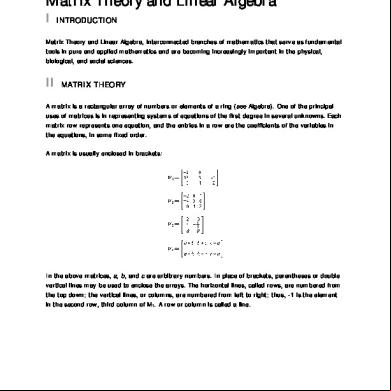
Matrix Theory And Linear Algebra 3z5l5e

Linear Algebra And Matrix Theory (nering).pdf 1m1z6w

E. D. Nering-linear Algebra And Matrix Theory-wiley (1976).pdf 3nw3a

Matrix And Tensor Calculus - Aristotle D. Michal 4l1i6a

Matrix E A Filosofia j4of

(e-book) Baldor Algebra z2l34

More Documents from "Julius" 3ph43

Federal Standard 209e Pdf 5m4t2j

Fast Fourier Transform And Its Applications Brigham Pdf 6s5e1t

Gst 103 Txt Book 4o4r4m

Ib Mathematics Sl Formula Booklet First Examinations 2014 4h4e5b

E. D. Nering-linear Algebra And Matrix Theory-wiley (1976).pdf 3nw3a

Molahonkey Song 4vd4g