Fea Theory 1n5u3

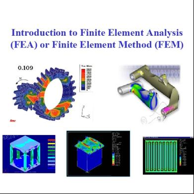
Introduction to Finite Element Analysis (FEA) or Finite Element Method (FEM)

Finite Element Analysis (FEA) or Finite Element Method (FEM) The Finite Element Analysis (FEA) is a numerical method for solving problems of engineering and mathematical physics. Useful for problems with complicated geometries, loadings, and material properties where analytical solutions can not be obtained.

The Purpose of FEA Analytical Solution • Stress analysis for trusses, beams, and other simple structures are carried out based on dramatic simplification and idealization: – mass concentrated at the center of gravity – beam simplified as a line segment (same cross-section) • Design is based on the calculation results of the idealized structure & a large safety factor (1.5-3) given by experience.

FEA • Design geometry is a lot more complex; and the accuracy requirement is a lot higher. We need – To understand the physical behaviors of a complex object (strength, heat transfer capability, fluid flow, etc.) – To predict the performance and behavior of the design; to calculate the safety margin; and to identify the weakness of the design accurately; and – To identify the optimal design with confidence

Brief History Grew out of aerospace industry Post-WW II jets, missiles, space flight Need for light weight structures Required accurate stress analysis Paralleled growth of computers

Common FEA Applications Mechanical/Aerospace/Civil/Automotive Engineering Structural/Stress Analysis 



Static/Dynamic Linear/Nonlinear

Fluid Flow Heat Transfer Electromagnetic Fields Soil Mechanics Acoustics Biomechanics

Discretization Simple Analysis

Complex Object (Material discontinuity, Complex and arbitrary geometry)

Real Word

Simplified (Idealized) Physical Model

Mathematical Model

Discretized (mesh) Model

Discretizations Model body by dividing it into an equivalent system of many smaller bodies or units (finite elements) interconnected at points common to two or more elements (nodes or nodal points) and/or boundary lines and/or surfaces.

Elements & Nodes - Nodal Quantity

Object

Elements

Nodes

Displacement

Stress Strain

Examples of FEA – 1D (beams)

Examples of FEA - 2D

Examples of FEA – 3D

Advantages Irregular Boundaries General Loads Different Materials Boundary Conditions Variable Element Size Easy Modification Dynamics Nonlinear Problems (Geometric or Material) The following notes are a summary from “Fundamentals of Finite Element Analysis” by David V. Hutton

Principles of FEA The finite element method (FEM), or finite element analysis (FEA), is a computational technique used to obtain approximate solutions of boundary value problems in engineering. Boundary value problems are also called field problems. The field is the domain of interest and most often represents a physical structure. The field variables are the dependent variables of interest governed by the differential equation. The boundary conditions are the specified values of the field variables (or related variables such as derivatives) on the boundaries of the field.

For simplicity, at this point, we assume a two-dimensional case with a single field variable φ(x, y) to be determined at every point P(x, y) such that a known governing equation (or equations) is satisfied exactly at every such point.

-A finite element is not a differential element of size dx × dy.

-A node is a specific point in the finite element at which the value of the field variable is to be explicitly calculated.

Shape Functions The values of the field variable computed at the nodes are used to approximate the values at non-nodal points (that is, in the element interior) by interpolation of the nodal values. For the three-node triangle example, the field variable is described by the approximate relation φ(x, y) = N1(x, y) φ1 + N2(x, y) φ2 + N3(x, y) φ3 where φ1, φ2, and φ3 are the values of the field variable at the nodes, and N1, N2, and N3 are the interpolation functions, also known as shape functions or blending functions.

In the finite element approach, the nodal values of the field variable are treated as unknown constants that are to be determined. The interpolation functions are most often polynomial forms of the independent variables, derived to satisfy certain required conditions at the nodes. The interpolation functions are predetermined, known functions of the independent variables; and these functions describe the variation of the field variable within the finite element.

Degrees of Freedom Again a two-dimensional case with a single field variable φ(x, y). The triangular element described is said to have 3 degrees of freedom, as three nodal values of the field variable are required to describe the field variable everywhere in the element (scalar).

φ(x, y) = N1(x, y) φ1 + N2(x, y) φ2 + N3(x, y) φ3 In general, the number of degrees of freedom associated with a finite element is equal to the product of the number of nodes and the number of values of the field variable (and possibly its derivatives) that must be computed at each node.

A GENERAL PROCEDURE FOR FINITE ELEMENT ANALYSIS • Preprocessing – – – – – –

Define the geometric domain of the problem. Define the element type(s) to be used (Chapter 6). Define the material properties of the elements. Define the geometric properties of the elements (length, area, and the like). Define the element connectivities (mesh the model). Define the physical constraints (boundary conditions). Define the loadings.

• Solution – –

computes the unknown values of the primary field variable(s) computed values are then used by back substitution to compute additional, derived variables, such as reaction forces, element stresses, and heat flow.

• Postprocessing –

Postprocessor software contains sophisticated routines used for sorting, printing, and plotting selected results from a finite element solution.