Tank Fea 334v5f
This document was ed by and they confirmed that they have the permission to share it. If you are author or own the copyright of this book, please report to us by using this report form. Report 3i3n4
Overview 26281t
& View Tank Fea as PDF for free.
More details 6y5l6z
- Words: 23,040
- Pages: 291
Copyright Notice © The material in this document is subject to copyright protection unless otherwise indicated. Much of the material contained herein was developed by the authors as part of the CCOPPS project, funded by the EU Leonardo programme. The University of Strathclyde is the formal copyright holder for this material. Permission has been granted by the University of Strathclyde for use of this material in this document. The collection of pressure vessel related photographs contains what is believed to be public domain and royalty free images. Where the source is known, this has been acknowledged. Should the copyright owner of any images in the collection wish these to be removed from the collection, then an e-mail to the following address will suffice: [email protected].
Acknowledgements Many people have contributed to the content of this resource, in varying degrees. I would therefore like to acknowledge this contribution in the following areas: Development of the CCOPPS work-based learning modules, which provided the two units contained herein, as well as the worked examples, tutorials and many of the photographs: Martin Muscat, University of Malta. Kevin Degiorgio, University of Malta. Johnny Zerafa , University of Malta. Hongjun Li, University of Strathclyde. Ian Holland, University of Strathclyde. Richard Cope, University of Strathclyde.
Development of the CCOPPS Educational Base: John McVee, retired consultant. Adib Becker, University of Nottingham. Trevor Hellen, retired consultant. Andy Morris, Eon Engineering UK. Steve Maddox, TWI. Manfred Zehn, Berlin University. Donald MacKenzie, University of Strathclyde. Jim Boyle, University of Strathclyde. Bobby Hamilton, University of Strathclyde. Alexander McIver Galloway, University of Strathclyde. David Nash, University of Strathclyde (also for the supply of photographs).
PREFACE The purpose of this resource book is to provide cost effective and convenient access to some of the material produced as part of the CCOPPS project, including the commercially available learning modules. Hopefully it will also act as an incentive for individuals to enrol on the work-based learning modules developed as part of CCOPPS and now offered by the University of Strathclyde (http://www.mecheng.strath.ac.uk/d.asp). The CCOPPS project had the following aims: • to maintain and develop the standard of professional development for engineers and analysts using analysis and simulation technology, in the power and pressure systems industry; • to encourage a greater diversity of learning and teaching delivery modes; • to promote lifelong learning. The resource book provides the following: 1. Access to the CCOPPS Educational Base in a manner that allows the individual to change and modify the content as desired (e.g. to add additional reference texts or to add additional competence statements). The original functionality and coverage of the CCOPPS Educational Base is retained. The reader can browse the 800 statements of competence covering 16 technical areas and use the hypertext links to identify reference texts that can be used to aid in the development of these competences. Individual records of each competence can be used to monitor personal development. 2. Access to 2 introductory units from the CCOPPS work-based learning modules : Introduction to Finite Element Analysis and Introduction to Design by Analysis – including 2 self-test quizzes. 3. Access to 9 system independent worked examples and tutorials. The focus is on the problem, idealisation and results. To access the solid models contained in the worked examples and tutorials you will have to use the freely available Adobe Reader 8.1 or later. This is available on the following link: http://www.adobe.com/s/. 4. Access to a collection of pressure vessel images, some of which form the basis of quizzes in the CCOPPS work-based learning modules. The majority however are simply nice photographs discovered in our search for educationally relevant images. Please note the copyright statement at the start of this document. This resource book is NOT aimed at a comprehensive coverage of pressure vessel design; does NOT provide a comprehensive coverage of FEA or DBA and does not contain coverage of specific commands on how to use any particular
finite element system. It is quite simply a collection of resource material in the pressure vessel and finite element areas, which will hopefully be of some use in personal development.
CONTENTS 1.
An Educational Base for the Use of FEA in the Power and Pressure Systems Industry. 1.1 1.2 1.3 1.4 1.5
Introduction Background Educational Rationale 1.2.1 Some reflections on “Experience” Using the Educational Base Areas of Competence Possible Further Developments 1.5.1 Available work-based learning material 1.5.2 Assessment of competencies
2.
A Practical Introduction to Finite Element Analysis.
3.
An Introduction to Pressure Vessel Design by Analysis.
4.
Worked Examples and Tutorials. 4.1 4.2 4.3 4.4 4.5 4.6 4.7 4.8 4.9
5.
Thick cylinder under various loading Small pipeline under in-plane-bending Cylindrical vessel with elliptical opening Elastic analysis of a flush cylindrical nozzle in a spherical vessel Large fabrication containing intersections Axisymmetric cylindrical vessel-skirt junction Thin un-welded flat end stress categorization Thick hemisphere plastic load analysis Torishperical head under internal pressure - buckling check (ASME VIII Div2 Part 5)
Pressure Vessel Related Images.
1.
An Educational Base for the Use of FEA in the Power and Pressure Systems Industry.
1.1 Introduction The CCOPPS Educational Base (available at http://www.ccopps.eu/) defines a set of recommended minimum educational requirements, for s of finite element analysis systems, in the Power and Pressure Systems Industry. The requirements provide a transparent, understandable description of the abilities that should be apparent in staff carrying out analysis and simulation in this industry sector. The Educational Base was developed as part of the EU-funded CCOPPS project (Certification of Competencies in the Power and Pressure Systems Industry) and it followed from a study of the educational and training needs of industry. The Educational Base is intended as guidance to those who are engaged in Continuing Professional Development, both at a personal level and at an organisational level. The base will be of use in staff development programmes as well as the design of educational resource material to deliver and assess the competencies expressed by these learning outcomes. In addition to enabling individuals and employers to establish whether they or their staff can meet these competence requirements, the base will provide links to resource material necessary to develop them. The Educational Base consists of a set of Competencies, expressed as Learning Outcomes, covering the following topic areas: Beams, Membranes, Plates and Shells Buckling and Instability Code of Practice Philosophy and Application Composite Materials and Pressure Components Creep and Time-Dependency Design by Analysis Dynamics and Vibration Fatigue Finite Element Analysis of Pressure Systems and Components Flaw Assessment in Pressure Components Mechanics, Elasticity and Strength of Materials Nonlinear Geometric Effects and Plasticity and Shakedown Pressure System Components and Fabrication Pressure Vessel Materials Thermo-Mechanical Behaviour All of the above are extensive areas of study in their own right and many researchers spend their entire professional lives working in only one or two of these. It is emphasized therefore that the competencies expressed in the
CCOPPS Educational Base represent a recommended minimum for practising engineers and analysts using FEM and who will invariably already have a first degree in engineering or a related discipline. For such engineers and analysts, moving into a new area of analyses, or perhaps needing to refresh existing competencies, this educational base and ing material, should provide a useful resource. It therefore focuses on aspects of technology that will be relevant to current engineering practice. The aim is that these should be sufficient to allow safe and effective use of modern analysis and simulation tools. They should also provide a basis for further educational development in these and related areas. They do not however consider the training needs of the particular application software being used, which is also clearly an important area of competence for effective use of the technology. The competencies outlined in the Educational Base do not address in a broad sense, underpinning subjects such as mathematics and computing, which might be expected to form part of an undergraduate education. In a similar vein, the Educational Base does not address wider aspects of an engineer’s professional development, such as management, finance, safety, ethics, environmental issues and inter-personal skills. In the UK, the output standards for accredited engineering degree programmes have been derived from a generic statement of learning outcomes adopted by the ECUK (former Engineering Council). Someone graduating from an accredited degree programme will, as a consequence, have competencies in these broader areas of an engineer’s development. It is also recognised that many unaccredited engineering degrees throughout the world, will also certainly address such areas, to varying levels. The route for the formation and development of engineers and analysts who use modern analysis and simulation tools to develop innovative, safe and competitive products in today’s marketplace are a progression of learning experiences beginning with an undergraduate degree, continuing through initial professional development in early employment and thereafter extending throughout their professional life. Once qualified, professional engineers and analysts today are expected to keep up to date by continued learning throughout (and in of) their career through Continuing Professional Development (D). Many of the competencies covered in the Educational Base would normally be developed as part of a formal postgraduate course, as part of a series of training courses or as part of on-the-job learning. 1.2 Background Educational Rationale The idea of an Educational Base providing a statement of the educational underpinning necessary for professional engineers is not new and most professional engineering bodies in the UK, will have a document containing such requirements. This document will be based on the ECUK generic statement of learning outcomes and will reflect their interpretation in the context of a specific engineering discipline (mechanical, electrical, civil etc). Satisfying the requirements of such an Educational Base will form part of the process of
becoming a member of a professional body. In the UK, the easiest way of satisfying these educational base requirements, is to graduate from an accredited University degree course, which has been designed to satisfy these requirements. Such degree programmes are regularly accredited by the appropriate professional engineering body and on approval, the University Department is sanctioned to deliver the accredited programme for a period of time – usually 5 years. This process involves all aspects of degree course design, delivery and assessment and includes consideration of intake and output standards. While the CCOPPS Educational Base has some similarities to the above, there are differences and it may be useful to consider these briefly. Firstly, the Educational Base statements guiding the design of undergraduate courses and hip of professional bodies are much broader in their scope and generally less specific in the statements of learning outcomes. For example the general learning outcomes will address practical skills in laboratories as well as transferable skills in working with others, information retrieval and planning selflearning. The specific learning outcomes will address the underpinning science (materials, mathematics, mechanics, thermodynamics, fluid mechanics, vibration, production and manufacture, control etc) as well as industrial context of the subject being studies. Design, creativity, project management, finance, environmental issues, sustainability, management, ethics, risk, health and safety are all indicative of the wider scope of such educational bases. Secondly, the individual modules forming part of a course of study will generally contain no more than half a dozen (often less) “higher level” learning outcomes. In this respect subject or module descriptors in degrees and diplomas may differ, with the latter containing more learning outcomes and often embodying different assessment regimes to certify competence. The reasons for this are partly historical. However, there is no doubt that assessing and re-assessing a large number of competencies in individual subject areas by the traditional examination methods inherent in existing University degree courses, would prove problematic. Assessing competencies using the appropriate tool is clearly important and much guidance is available for staff involved in this process. However the CCOPPS project was not concerned with the practicalities and constraints within any educational system or sector and therefore had the luxury of developing a detailed list of competencies that can be used in a formative sense by individuals engaged in continuous professional development in the work place. In this case, self-assessment or assessment by a mentor or line-manager is likely to be the order of the day, rather than by means of the invigilated examination systems typical of University systems. This obviously does not preclude use of such learning outcomes in a formal assessment system, but in this case the development of module descriptors for use as part of a formal degree programme would almost certainly involve a focus on delivery and formal assessment of a fewer selected number of “higher level” learning outcomes.
It may also be useful at this point to introduce some of the educational rationale behind the use of statements of competence or learning outcomes in an educational base. Learning outcomes in this context are statements of what an analyst should be able to do at the end of a programme of learning. The emphasis on doing is what distinguishes a learning outcome approach from one based on more intangible ideas related to educational aims, objectives and a list of syllabus content. For some, the main problem with such a syllabus is that it can give little or no indication of depth or approach to any particular topic and also time spent. Many academics in fact value such looseness and academic freedom, to place emphasis where they see fit. There can also be course management advantages and disadvantages associated with such freedom. However, in of providing the employer, or the student with details of what competences they should have at the end of the course, it is argued that it is less than satisfactory, even when notional hours are provided in such syllabi. A list of detailed learning outcomes, on the other hand, provides employers and students with useful information on what competences should be in place at the end of the learning experience. Learning outcomes also help instructors to design and select suitable resource material more effectively, to select the appropriate method of delivery and to select appropriate assessment methods. It might also be argued that learning outcomes are particularly useful where resource material and learning activities are going to be designed by many different people, in order to be used by others, perhaps in a distributed environment. This point is particularly relevant in today’s diverse and distributed finite element community and the way that this Educational Base may be used in the development and selection of ing resource material. It is concluded therefore that learning outcomes or statements of competence are the natural way to frame educational requirements in this environment. In the present context however, we are interested in identifying desirable learning outcomes or competencies for the various s of the technology undertaking the different analysis types. The specified list must inevitably strike a balance between the level of prescriptive detail and the general indications of competency required. Issues associated with the assessment, re-assessment, quality and retention of these competences are clearly important educational considerations. These issues are not the main focus of this project, although they are addressed briefly, later in this section. It is also emphasized that effective course design, in an academic environment, would naturally involve selection of the appropriate assessment tools and also identification of the most appropriate methods of delivery of the course content, with a view to satisfying the learning outcomes. It is also argued that, given the various levels in the cognitive area, discussed below, the process of identifying suitable material (text books, short courses, web-based learning modules etc), that can be used in satisfying the learning outcomes, should involve more than simply identifying textual information aimed solely at imparting knowledge. Any material specified should allow those using it
to develop competence in the so-called higher cognitive levels (if not also in the affective and psychomotor areas), even if only in a formative manner. This latter point emphasises the need for diversity in resource material, including workbooks, case studies, worked examples, tutorials etc. Various attempts have been made at systematically describing different categories and levels of learning and it has long been postulated that there are 3 broad categories: • Cognitive - which deals with acquisition and use of knowledge. • Affective - which deals with attitudes and value judgements. • Psychomotor - which deals with manipulative skills. It has been accepted that University level education, in engineering in general, traditionally gives much more attention to the cognitive area. The Cognitive Area The following six cognitive sub-areas are typically presented as increasing in level from knowledge to evaluation. The engineering problem-solving and design activity, typical in the University sector, is clearly associated with the so-called higher cognitive levels, while building on a solid foundation of knowledge and understanding. Knowledge is the ability to recall information, to describe known ways of dealing with this information or to state previously learned general principles or theories. Comprehension is the ability to demonstrate understanding by interpreting information or extrapolating from given data in order to determine likely implications or effects. It is common for those not involved in education to assume that the term knowledge includes comprehension, but clearly this need not be so. For example, it may be argued that many pressure vessel designers routinely use Code formulae with little comprehension of how such formulae were derived and the assumptions inherent in their development. Codes of Practice will typically avoid the possible serious consequences of this state of affairs by including a range or scope statement - however, this clearly does not imply comprehension on the part of the . In fact, it is possible that some noneducationalists will effectively assume the term knowledge to include the entire cognitive area. Application is the ability to apply principles to particular situations. Analysis is the ability to break a problem down into its constituent parts to seek clarification, to identify structure and relationships between parts. Synthesis is concerned with bringing together a number of facts and ideas to create a new approach or procedure. Evaluation deals with judgements about the value of materials, methods, solutions and designs. Academics typically will use different assessment instruments to ascertain competences in each of these areas. For example computer-based multiple choice questions are commonly used to assess knowledge,
comprehension and to a lesser extent application, whereas typical engineering problem solving exam questions can address all of the above, as can project work. Work-based projects are an excellent vehicle to develop and reinforce competencies, in the so-called higher cognitive levels of application, analysis, synthesis and evaluation in particular. As shown in Figure 1, the statements of competence in each topic covered by the CCOPPS Educational Base, have been conveniently grouped into each of the above cognitive areas.
Figure 1:
Sample Statements of Competence from the CCOPPS Educational Base
The Affective Area It is true to say that much less attention is given in engineering higher education to the assessment of attitude and value judgements by students - unlike medicine for example, where students must demonstrate attitudes, ethical development and values desirable in a medical practitioner. The Psychomotor Area The importance of psychomotor skills varies across disciplines from music to social studies. In engineering, they play some importance in laboratory work, including keyboard skills and the use of application software such as finite element systems.
The learning outcomes contained in the CCOPPS Educational Base primarily address the cognitive area. Also inherent in today’s holistic and increasingly global view of education is the concept of level and when used to construct a degree award it is common to associate learning outcomes with a level of study. A number of generic level definitions exist across the Higher Education sector and efforts are underway to produce a standard model. These efforts are often driven by the need to facilitate mobility (nationally and internationally) amongst students through some form of Credit Accumulation and Transfer System. The diversity of education systems throughout the world makes the realisation of this particularly challenging. It should be recognised that the level of study is different from the level of performance or standard of attainment achieved in fulfilling the learning outcome. When used as part of a formal award such as a degree, learning outcomes would normally be accompanied by a threshold statement and grade indicators. These would in turn be used by assessors to categorise and rank student performance. To illustrate this further development of learning outcomes, it may be useful to consider an example. Consider the learning outcome Employ a range of postsolution checks to determine the integrity of FEA results. A minimum acceptable performance or threshold statement associated with this might be Use 2 or 3 post-solutions checks to determine the integrity of FEA results. An “A grade” or comprehensive performance on the other hand might be to Identify the most appropriate post-solution checks and use them to specify the integrity of FEA results, with a full justification of choices. It should be recognised that even with this level of detail, there is still scope for any assessor to exercise their professional judgement in setting any examination instrument and in interpreting level of achievement. It has already been indicated however that the Educational Base will find use in an individual assessing their own competence level in an informal manner or in his manager attesting to a member of staff’s competence informally, as part of an internal system of staff development, or even in the development of a of Suitably Qualified Staff as part of an internal Quality Assurance System. In these instances, s may not be interested in performance level indicators. Performance level statements for Threshold and Comprehensive have however been included in the Educational Base, for completeness and to assist with adoption and integration into formal educational programmes. These are included on the Individual Competence Record Sheet associated with each statement of competence in each topic area, as shown in Figure 2. These sheets may be printed out to enable individuals to keep a record of their achievements.
Figure 2:
Individual Record Sheet from the CCOPPS Educational Base
To encourage this latter use of the statements of competence encomed in the CCOPPS Educational Base, it will prove useful to present the material with reference to a particular educational model. The model chosen for this purpose is the developing European Higher Education Area which embodies the European Credit Transfer Scheme. The framework for the EHEA consists of three main cycles. First cycle qualifications relate to bachelor or undergraduate degrees (with and without honours). Second cycle qualifications relate to Masters degree level and third cycle to Doctoral degrees. This system is based on the concept that one academic year consists of 60 credits worth of learning or student effort hours. The thinking behind the concept of a student effort hour and how many should constitute an academic year for a full-time student is not discussed here. Suffice to say that any concept of student credit will stem from such
considerations. Student effort hours would normally include private study time as well as formal class , laboratories, tutorials and assessments. In the European Qualifications Framework there are 8 levels and level 6 corresponds to cycle 1, level 7 to cycle 2 and level 8 to cycle 3. Although an introduction to the study of finite element analysis and pressure system design may appear in cycle 1 degrees, these subjects and related topics such as shells, fracture mechanics, plasticity, creep, shakedown etc are more often found in cycle 2 degrees. In the UK, study in depth in these areas would normally be found in MSc programmes as opposed to integrated MEng degrees. Such MSc’s however are few in number. More often, coverage of these topics in any depth will be delivered in short intensive courses, which normally would not form part of any formal degree award. In some disciplines however, postgraduate awards (typically MBAs) may be found, where the method of delivery is short intensive courses. In summary therefore, the learning outcomes contained in the CCOPPS Educational Base are mainly at levels 7 and 8, although there are also outcomes relating to a revision of underpinning material at level 6. The two ing webbased learning modules would typically represent 20 credits in the European credit model (i.e. a third of an academic year’s effort) at level 7. While such considerations may be of little interest to someone simply using the Educational Base to guide informal personal development, such rationale will prove useful to anyone considering using it to construct formal modules for an award. The EQF level for each learning outcome has also been added to the Educational Base. Also included is an indication as to whether the learning outcome / statement of competence is considered appropriate to an analyst at Standard or Advanced level. The concept of Standard and Advanced analyst is currently embodied in a model for a NAFEMS ed Analyst Scheme. The idea of Standard and Advanced analysts is somewhat similar to the notion of Incorporated Engineer or Chartered Engineer in the UK. It may also be observed that the learning outcomes categorised as Advanced are mainly associated with the higher cognitive levels. It is argued that the CCOPPS Educational Base, framed in of competence statements, could form a robust and philosophically sound basis for a ed Analyst Scheme. It is noted that NAFEMS are in fact considering the possibility of generalising the CCOPPS Educational Base and in turn use this as the basis for specifying and assessing analysts competence. 1.2.1 Some reflections on “Experience” Application for hip of a professional body will often have requirements in addition to satisfying the Educational Base - which is primarily taken as a measure of the adequacy of someone’s underpinning background engineering education. In particular, applicants generally have to undergo a period of Initial Professional Development and to demonstrate sufficient experience in a position of professional responsibility. There is invariably a requirement to supply details of professional experience – in particular, details of responsibility
(management, projects, budgets, key achievements, demonstration of engineering expertise). This latter requirement is often assessed at a Professional Review Interview after submission of a Professional Review Report. The current NAFEMS ed Analyst Scheme also places emphasis on experience - in this case conducting various types of analyses in a particular branch of industry and in planning and managing FEA projects and resources. It may be useful therefore to reflect on the meaning of experience in a wider educational sense, in relation to the formation of an engineer or analyst. A simple definition of experience is practical knowledge gained by trial or practice. Having an education and never having put it into practice in a real industrial context would be regarded as a less than ideal situation for an engineer. Learning from idealised problems and benchmarks are essential as part of the educational process, but at the end of the day, the focus necessary when faced by a real application, in an industrial environment, is recognised as highly beneficial in many ways. The term experience is often used loosely and it is generally thought of as good, but its quality is very rarely measured. The observations may be made that experiences can be bad as well as good; that having experience indicates nothing in itself about particular outcomes or the quality of any relevant outcomes from such experience; that someone can have the same experience a hundred times and learn very little that is new. In this latter case however, it is also recognised, from an educational viewpoint, that repetitive experience is a mechanism for committing knowledge to long-term memory and is therefore generally of benefit. In of developing what educationalists refer to as deep learning, it is accepted that practice and experience of a range of problems covering a wide range of possible variables is a necessary ingredient in the process. While it is true to say that an analyst’s industrial experience is never subjected to the same formal assessment process as their education, the argument might be made that the fact that the analyst remains in employment is testimony to satisfactory experience at least. A reference from an employer or statement by a referee might be regarded in a similar way, in spite of the fact that it would not be uncommon for an employer or referee to have a vested interest in the outcome of an individual’s application to a professional body. This may often be satisfactory for the purpose, but it is important to realise that this situation is obviously not as rigorous as an educational process that involves assessment of stated competences. It is however a fact of life that the further one progresses in a career, the more one is judged by actual achievements and the testimony of others, rather than formal assessment of competencies. When combined with a formal interview by a of peers, structured around a technical submission, the rigour and integrity of the process of examining experience and achievements is clearly enhanced.
The assessment of experiential learning is also something that has taxed the minds of academia in recent years, in an effort to award appropriate credit towards an academic award for prior experiential learning. The interest in this area is generally to facilitate advanced entry into formal educational programmes for mature students. No doubt much useful guidance is available in the literature on this matter. However, it is likely that the process involves subjective judgement rather than any kind of formal assessment, such as a written or even oral examination. How then should requirements regarding experience in the professional development of analysts be stated? For example, should someone become a advanced analyst by accumulating repetitive experience on the same type of jobs - that may in themselves be relatively undemanding? Simply requiring an advanced analyst to have more experience would seem to be a rather woolly and ill-defined requirement (particularly if measured by say a simple accumulation of points gained by conducting the same or similar analyses). Clearly any experiential statement requires some form of context and qualification. This issue also raises fundamental questions relating to the purpose and use of any statement of education and professional development in the finite element area. For example is the purpose to draw up a professional development framework: • that may be adopted by some regulatory body? • that courts might use when assessing professional negligence cases? • that companies might refer to when placing contracts or employing staff? • that employers and s of the technology might simply refer to in of professional development? Clearly the first three demands more rigour in assessing individual competence than the latter. Arguably it should be possible to frame the result of any industrial experience as a learning outcome or statement of competence, if we view experience as part of an educational process i.e. to specify what has been the educational outcome of this experience. In this regard the extensive learning outcomes embodied in the CCOPPS Educational Base already reflect the outcome of relevant experiential processes for the analyst. However if we also recognise experience as a context of application in an industrial environment, then it is clear that this is where the benefit of any experiential requirement lies. It is therefore recommended that the higher level learning outcomes in the Educational Base be developed in an industrial context wherever possible. It is also recommended that any definition of an advanced analyst be based solely on achievement of these learning outcomes. Clearly there is still a requirement for a scope statement outlining the range of competencies, at what level and in what industry sector. Having competence in finite element application in the aircraft industry does not necessarily indicate the same level of competence in the power and pressure systems industry or biomedical device
sector. However, it is noted that industrial sector relevance can also be addressed by competency statements, such as those expressed in the topics: Code of Practice Philosophy and Application Design by Analysis Pressure System Components and Fabrication Pressure Vessel Materials The grouping of statements of competency in such industry-specific categories, is the vehicle to allow a generalisation of the CCOPPS Educational Base so that it has direct relevance to other sectors. 1.3 Using the Educational Base The Educational Base is available with this resource book and s are able to access all areas covered. s are also able to print out the lists of learning outcomes / statements of competence, as well as the individual record sheets for each competence. This therefore will allow analysts to maintain their own personal development record and to plan accordingly. Unlike the on-line version of the Educational Base, s of the version accompanying this resource book will also be able to modify the base. As shown in Figures 1 and 2, the sheets printed out will contain the following information: • • • • • •
•
A category and code number for each learning outcome or statement of competence. A statement of each learning outcome / statement of competence. A Threshold and Comprehensive performance interpretation of each learning outcome. An indication of the European Qualification Framework (EQF) level for each learning outcome and whether the outcome is considered to be appropriate to a Standard or Advanced level of analysis. A reference to ing resource material that can be used to facilitate the development of each learning outcome. Tick boxes to indicate whether the competence expressed in each learning outcome has been attained and whether this has been done informally (e.g. by self learning or a short course with no examination) or formally (e.g. by an examined programme of learning). A signature box to allow a manager to attest to such achievement.
Most of the above information is for the use of the person engaged in personal development. The latter two items of information are to encourage and facilitate the development of company staff development schemes and perhaps a future ed Analyst Scheme. 1.4 Areas of Competence
The focus of this Educational Base is the use of finite element methods in of the design and analysis of pressure systems and components. The learning outcomes / statements of competence have been grouped into the 16 areas shown in Figure 3. This figure shows the web-based interface to the CCOPPS Educational Base.
Figure 3:
Web-based Interface to the CCOPPS Educational Base
These categories include specific outcomes relating to finite element analysis as well as a wide range of topics necessary to safe and effective use of this technology. The areas were identified in a study of Industry Needs, also completed as part of the CCOPPS project. In developing the learning outcomes in these ing topic areas, the goal was to provide sufficient background to finite element analysis. For this reason, non-numerical and other numerical methods have not been addressed.
Development of the learning outcomes embodied in these areas, invariably would not represent the same amount of student effort hours and a number of them could be combined to provide similar levels of educational content, if being used in a formal educational programme. The Educational Base has been developed in a manner that allows future expansion and modification of the learning outcomes and ing topic areas. 1.5 Possible Further Developments 1.5.1 Available work-based learning material The CCOPPS project developed web-based learning material in Design by Analysis and Finite Element Analysis of Pressure Systems and Components. This material will allow engineers engaged in D to develop their competence in these specific areas. Each learning outcome in the Educational Base in these areas will provide reference to the specific area of the web-based learning material that addresses the particular competence. The webbased learning material will also contain self-test questions, worked examples, tutorials and suggestions for further analysis. In developing the web-based learning material, attempts have been made to facilitate an informal, exploratory approach to the material. It is anticipated that these modules will also act as exemplars for the development of web-based learning material in the other topic areas, as future funding becomes available. The Educational Base however provides references to conventional text-based resource material that can also be used to develop competencies in all areas. This resource book contains two introductory units from these work-based learning modules. 1.5.2 Assessment of competencies The web-based learning modules developed as part of the CCOPPS project will provide self-test resource material for the informal formative assessment of the competencies expressed by the various learning outcomes in the Educational Base. This resource book contains two self-test quizzes from these work-based learning modules. The formal summative assessment of competencies, as typified by invigilated University examinations, will be addressed to some extent through the production of threshold and comprehensive statements for each outcome. It should not prove difficult therefore, to use the Educational Base for the development of modules leading to formal academic awards.
2.
A Practical Introduction to Finite Element Analysis.
Before investigating the unit from the CCOPPS learning module, please have a look at the ree file on the following link: http://personal.strath.ac.uk/j.wood/CCOPPS_FEA/ree.htm This unit from the CCOPPS Introduction to FEA of Pressure Systems and Components workbased learning module is available by simply clicking on the link below: http://personal.strath.ac.uk/j.wood/CCOPPS_FEA/home.htm As can be seen, the structure of the full work-based learning module is available, although access is restricted to this unit only. This enables readers to browse the module content and structure to some extent, before ing for the full module. Registration also allows access to the course tutors for 5 months. The Element Selection self-test quiz from the Basic Modelling unit in this module is available by clicking on the following link: http://personal.strath.ac.uk/j.wood/CCOPPS_FEA\quiz\Element_Selection\eleme nt_selection_quiz.html
3.
An Introduction to Pressure Vessel Design by Analysis.
Before investigating this unit from the CCOPPS learning module, please have a look at the ree file on the following link: http://personal.strath.ac.uk/j.wood/CCOPPS_FEA/ree.htm This unit from the CCOPPS Introduction to DBA of Pressure Systems and Components workbased learning module is available by simply clicking on the link below: http://personal.strath.ac.uk/j.wood/CCOPPS_DBA/home.htm As can be seen, the structure of the full work-based learning module is available, although access is restricted to this unit only. This enables readers to browse the module content and structure to some extent, before ing for the full module. Registration also allows access to the course tutors for 5 months. The DBA Basics self-test quiz from the Introduction to Pressure Vessel DBA unit in this module is available by clicking on the following link: http://personal.strath.ac.uk/j.wood/CCOPPS_DBA/Quiz\Quiz_DBA_basics\Quiz_ DBA_basics.html
4.
Worked Examples and Tutorials.
The following are a selection of the worked examples and tutorials available in the work-based learning modules developed as part of CCOPPS and now offered by the University of Strathclyde. The following link provides further details on costs and how to enrol: (http://www.mecheng.strath.ac.uk/d.asp). The modules contain a further 55 worked examples. To access the solid models contained in the following worked examples and tutorials you have to use the freely available Adobe Reader 8.1 or later: http://www.adobe.com/s/.
WORKED EXAMPLE DEFINITION Number:
Title:
CCOPPS_BMW1
Thick cylinder under various loadings
Page 1 of 5
Date: 20th May 2009
Statement of Purpose: The main purpose of this example is to demonstrate the use of 2D planar elements and axisymmetric elements to model a long thick cylinder under different loadings: internal pressure, non-uniform temperature field, rotation about its centre line and a shrink fit. Geometry:
a=0.1m, b=0.2m, c=0.3m
WORKED EXAMPLE DEFINITION
Page 2 of 5
Analysis Type(s):
Material:
Linear material, static, small displacement.
Steel, with Young’s Modulus = 209GN/m2; Poisson’s Ratio = 0.3; Density = 7800kg/m3, thermal expansion coefficient = 1.3e-5/degK.
Loading:
Boundary Conditions:
Case 1: a uniform internal pressure of 1 MPa.
Symmetry boundary conditions are applied on planes of symmetry.
Case 2: a rotation ω=1000 rad/s about its axis. Case 3: temperature Ti=1°C on the inner surface and To=0°C on the outer surface. The steady state through thickness temperature distribution is given by the function:
T=
Ti b ln b r ln a
Case 4: the interference shrinkage, δ=1E-4m, at the bore of the outer cylinder i.e. inner radius=0.1999m.
WORKED EXAMPLE DEFINITION
Page 3 of 5
Target Solution Quantities Required for Comparison: Loading case 1 (Internal Pressure): The radial stress distribution is described by [1]:
⎡ b2 ⎤ ⎢1 − 2 ⎥ ⎣ r ⎦
σr =
pa 2 b2 − a2
σh =
pa 2 ⎡ b 2 ⎤ ⎢1 + ⎥ b2 − a2 ⎣ r 2 ⎦
and hoop stress distribution by:
Loading case 2 (Rotation About Axis): The radial stress [1]:
σr =
a 2b 2 3+v⎛ 2 ⎜⎜ a + b 2 − r 2 − 2 8 ⎝ r
⎞ 2 ⎟⎟ ρω ⎠
occurs at r = ab = 0.1414 m The hoop stress is maximum at the inner edge:
σh =
3+v⎛ 2 1 + 3v 2 a 2 b 2 ⎜⎜ a + b 2 − r + 2 8 ⎝ 3+v r
⎞ 2 ⎟⎟ ρω ⎠
Loading case 3 (Thermal Stress): The radial stress distribution is described by [1]:
σr =
⎡ b a2 − − ln b⎢ r b2 − a2 2(1 − v ) ln ⎣ a EαTi
⎛ b2 ⎜⎜1 − 2 ⎝ r
⎞ b⎤ ⎟⎟ ln ⎥ ⎠ a⎦
⎛ b2 ⎜⎜1 + 2 ⎝ r
⎞ b⎤ ⎟⎟ ln ⎥ ⎠ a⎦
and hoop stress distribution by:
σh =
⎡ b a2 1 ln − − b⎢ r b2 − a2 2(1 − v ) ln ⎣ a EαTi
Loading case 4 (Shrink Fit): The pressure between the cylinders [1]:
pc =
Eδ (b 2 − a 2 )(c 2 − b 2 ) = 24.49 MPa b 2b 2 (c 2 − a 2 )
The radial stress at the bore of the outer cylinder = − p c The hoop stress at this position σ h =
p (b 2 + c 2 ) c2 − b2
Idealisations: The cylinder is long enough and loadings are symmetric so that the cross-section remains plane during deformation. Due to the symmetry, only a quarter of the cross section need be modelled as shown in the following figure. An axisymmetric idealisation is also possible as shown.
WORKED EXAMPLE DEFINITION
Page 4 of 5
Further Considerations: 1. Reduce the model to say a 10 degree sector (Mesh ABFE) and apply suitable constraints along edge EF. Compare results with previous model. 2. If an axisymmetric model is used, what boundary conditions should be applied on edges IJ and GH for plane stress and plane strain cases, respectively?
WORKED EXAMPLE DEFINITION
Page 5 of 5
3. Which idealisation is better, axisymmetric or planer? Why might this be? 4. Examine the effects of varying aspect ratio in the hoop direction. 5. How much would you have to heat the outer cylinder up by so that it just slipped onto the inner cylinder, for load case 4? 6. What rotational speed would cause loss of at the interface in load case 4. 7. Identify the axial stress distribution for each loading case.
Useful references: 1. S. Timoshenko, Strength of Material, Part II, Advanced Theory and Problems, 3rd Edition, D. Van Nostrand Co., Inc., New York, NY, 1956, pp. 208, loading case 1, pp. 217, loading case 2, pp. 231, loading case 3, pp. 211, loading case 4.
SOLUTION Page 1 of 13
Number: CCOPPS_BMW1
Title: Thick cylinder under various loadings
Date: 20th May 2009
Idealisation: The cylinder is long enough and loadings are symmetric so that the cross-section remains plane during deformation. Due to the symmetry, only a quarter of the cross section need modelled ABCD as shown in the following figure. A smaller sector model is possible, although this would involve the imposition of constraints in a non-global axis set. Both 2D plane stress and plane strain elements may be used for the 90 degree 2D solid model, although only the plane strain idealization is equivalent to the axisymmetric model shown. An axisymmetric idealisation is also possible as shown. Again a single element wide idealisation should be possibly in the absence of end effects.
SOLUTION Page 2 of 13
Mesh: Load case 1: uniform internal pressure Axisymmetric model
2D planar model (Plane Stress or Plane Strain)
SOLUTION Page 3 of 13
Load case 2: rotation & load case 3: temperature Axisymmetric model
2D planar model
Load case 4: shrink fit Axisymmetric model
System and Element(s) Used: ABAQUS version 6.6-1 Axisymmetric model: An 8-node second-order element with reduced integration, CAX8R 2D planar model: An 8-node bi-quadratic plane stress quadrilateral element with reduced integration, S8R (stress in normal direction is zero) and an 8-node bi-quadratic plane strain, quadrilateral, reduced integration element, E8R (strain in normal direction is zero). Surface to surface defined with default properties. Results for Comparative Target Solution Quantities:
SOLUTION Page 4 of 13
Load case 1: a uniform internal pressure of 1 MPa.
Figure 1 Mesh convergence study for the axisymmetric model, load case 1
Figure 2 Hoop stress fringe plot for the axisymmetric model, load case 1
Figure 3 Radial stress fringe plot for the axisymmetric model, load case 1
SOLUTION Page 5 of 13
From the previous convergence study, it was found that 2 elements provided a reasonable estimate of maximum values, The model with six elements in the radial direction is used to compare results with theory. For the 2D planar model, a mesh convergence study was also carried out by fixing the number of elements in the radial direction at 6 and increasing the elements in the hoop direction. This study is however providing more of an indication of the effects of element distortion than mesh refinement.
Figure 4 Mesh convergence study for the 2D planar model, load case 1
Figure 5 Hoop stress fringe plot for the 2D planar model, load case 1 It is clear from the above figure that the stress fringe plot is not quite smooth. This may be due to the typical variation observed between corner and midside node results. This difference will reduce with mesh refinement in the hoop direction. Such variations are also sometimes a result of fringe plotting algorithms. A check of corner and nodal values will help to confirm the cause.
SOLUTION Page 6 of 13
Figure 6 Radial stress fringe plot for the 2D planar model, load case 1 As the same results were obtained for plane strain and plane stress elements, in the Figure 7, only one set of the results are plotted with the name “2Dplanar”.
Figure 7 Comparison with theorectical results for load case 1
SOLUTION Page 7 of 13
Load case 2: a rotation ω=1000 rad/s about its axis.
Figure 8 Mesh convergence study for the axisymmetric model, load case 2
Figure 9 Hoop stress fringe plot for the axisymmetric model, load case 2
Figure 10 Radial stress fringe plot for the axisymmetric model, load case 2
SOLUTION Page 8 of 13
From the axisymmetric model convergence study, it is found that six elements along radial direction are able to provide excellent results. For the 2D planar model, a mesh convergence study was also carried out by fixing the number of elements in the radial direction at 6 and increasing the elements in the hoop direction. No. of elements Max. radial stress (Mpa) Error_r (%) Max.hoop stress (Mpa) Error_p (%) 4 3.53E+07 5.35 2.86E+08 2.88 6 3.40E+07 1.73 2.81E+08 1.08 8 3.37E+07 0.72 2.79E+08 0.36 10 3.35E+07 0.24 2.78E+08 0.14 12 3.35E+07 0.00 2.78E+08 0.00 Table 1 Mesh convergence study for the 2D planar model, load case 2
A coarse mesh with six elements in the hoop direction is used in the following analysis.
Figure 11 Hoop stress fringe plot for the 2D planar model, load case 2
Figure 12 Radial stress fringe plot for the 2D planar model, load case 2
SOLUTION Page 9 of 13
3.00E+08 2.50E+08 2.00E+08 Theory_radial Theory_hoopl Axisym_hoop Axisym_radial plane_strain_hoop plane_strain_radial plane_stress_hoop plane_stress_radial
) 1.50E+08 m / N ( ss e rt 1.00E+08 S
2
5.00E+07 0.00E+00 0.08
0.1
0.12
0.14
0.16
0.18
0.2
0.22
‐5.00E+07 Radial distance (m)
Figure 13 Comparison with theoretical results for load case 2 Load case 3: steady state temperature distribution through thickness By comparing the analytical stress solutions for load case 1, 2 and 3 and mesh convergence studies for load case 1 and 2, it is reasonable to say that 6 elements along radial direction is able to produce a satisfactory solution. The figure 14 proves our judgement. The numerical hoop stress results show a large discrepancy from the analytical solution. A 10 percent error was predicted by the axisymmetric model. Hence a finer mesh with 10 elements in the radial direction was created. In the fine planar mesh, 10 elements in the hoop direction were used. Figure 15 presents the comparison with theoretical results using fine meshes.
SOLUTION Page 10 of 13
2.00E+06 1.50E+06 1.00E+06 5.00E+05 ) 0.00E+00 m / 0.08 (N s s ‐5.00E+05 re tS ‐1.00E+06
2
0.1
0.12
‐1.50E+06 ‐2.00E+06 ‐2.50E+06
0.14
0.16
0.18
0.2
0.22
Theory_radial
Theory_hoopl
Axisym_hoop
Axisym_radial
plane_stress_hoop
plane_stress_radial
plane_strain_hoop
plane_strain_radial
‐3.00E+06
Radial distance (m)
Figure 14 Comparison with theoretical results for load case 3, 6 elements in radial direction. 2.00E+06 1.50E+06 1.00E+06 5.00E+05 ) 0.00E+00 m / 0.08 N ( ‐5.00E+05 ss e rt S ‐1.00E+06
2
‐1.50E+06 ‐2.00E+06 ‐2.50E+06
0.1
0.12
0.14
0.16
0.18
0.2
0.22
Theory_radial
Theory_hoopl
Axisym_hoop
Axisym_radial
plane_stress_hoop
plane_stress_radial
plane_strain_hoop
plane_strain_radial
‐3.00E+06
Radial distance (m)
Figure 15 Comparison with theoretical results for load case 3, 10 elements in radial direction.
SOLUTION Page 11 of 13
Figure 16 Radial stress fringe plot for the axisymmetric model, load case 3
Figure 17 Hoop stress fringe plot for the axisymmetric model, load case 3 Load case 4: shrink fit
SOLUTION Page 12 of 13
Figure 18 Radial stress fringe plot for the axisymmetric model, load case 4
Figure 19 Hoop stress fringe plot for the axisymmetric model, load case 4
Analytical solution
Axisymmetric model (error %)
24.49 MPa
24.48 MPa (0.04%)
2D solid model (error %) Plane stress
Plane strain
24.7 MPa (0.8%)
27.2 MPa (11%)
Figure 20 Comparison with theorectical results for load case 4 Relevant Codes of Practice, Industry Standard and/or Statement of Assessment Criteria:
Description of Results Post-processing (where relevant):
Conclusion(s): In this example, a thick cylinder was modelled under four different loadings: internal pressure, non-uniform temperature field, rotation about its centre line and a shrink fit.
SOLUTION Page 13 of 13
Load case 1 (Internal Pressure): The axisymmetric idealisation, with Plane Strain constraints, provides good agreement with theory. Both 2D plane stress or plane strain elements also provide excellent results, as the hoop stress and radial stress do not depend on the elongation εy. Load case 2 (Rotation): The axisymmetric idealisation, with Plane Strain constraints, provides good agreement with theory. The radial stress results from all the 2D planar models are in good agreement with the theoretical solution. For the hoop stress distribution, the plane strain element model shows a little deviation (6.6%), for the mesh used. Load case 3 (Temperature): The axisymmetric idealisation, with Plane Strain constraints, provides good agreement with theory. Not surprisingly, a large discrepancy occurs between the Plane Strain analytical solution and results predicted by the Plane Stress model, indicating that the assumption that the axial stress is planar and zero, is not suitable for this case. Load case 4 (Shrink Fit): The axisymmetric idealisation, with Plane Strain constraints, provides good agreement with theory. If you are interested in analysing this type of structure and component, it is highly recommended that you repeat this exercise with your own FE system and elements therein.
WORKED EXAMPLE DEFINITION Number:
Date:
Title:
CCOPPS_BMW2
Page 1 of 3
Small pipeline under IPB
20th May 2009
Statement of Purpose: The main purpose of this example is to demonstrate the use of thin shell elements to model a small pipeline with an elbow. In addition, simple beam elements with a “flexibility factor” and “stress intensification factor” are used to quantify the global effect of ovalization.
Geometry:
a=250mm r=11.4mm t=0.6mm, R=100mm
WORKED EXAMPLE DEFINITION
Page 2 of 3
Analysis Type(s):
Material:
Linear material, static, small displacement.
Steel, with Young’s Modulus = 194GN/m2; Poisson’s Ratio = 0.3.
Loading:
Boundary Conditions:
Case1: Unit inward displacements imposed on both ends of the structure.
Shell model: Symmetry boundary conditions are used on the two symmetry planes of the pipe line, the intrados node of the bend on the symmetry plane is fixed to prevent free body movement. Beam model: symmetry boundary condition is on the cross-sectional symmetry plane.
Target Solution Quantities Required for Comparison: Compare reaction forces and bending stresses using different models.
Idealisations: Since the pipe mean radius to thickness ratio is 19, thin shell element would be appropriate. Due to geometry symmetry, a quarter of the pipeline is modelled in a shell element model. The schematic representation of the FE idealisation is shown as below.
An alternative method of modelling the pipeline is to use beam elements. To include the effects of ovalization, reduced bending stiffness should be implemented in elements of the elbow. These elements are highlighted in green colour in the following figure.
The value of the reduced stiffness was obtained from the equation:
k=
1.66
λ
where
λ=
Rt r 2 1 −ν 2
WORKED EXAMPLE DEFINITION
Page 3 of 3
R is the radius of the curved section, r is the mean radius of the pipe, t is the wall thickness of the pipe, and v is Poisson’s ratio. The reference for the above equation is Dodge and Moore [1]. This gives a value of k = 3.43, so the bending stiffness was reduced by a factor of 3.43. This was done by reducing the thickness of the bend. The other approach to reducing the bending stiffness is to reduce the Young’s modulus. The flexibility characteristic, flexibility factor and stress intensification factor are calculated as below according to ASME B31.1-2007. Flexibility characteristic,
Flexibility factor,
k =
λ =
Rt r2
1.65
λ
Stress intensification factor,
i=
0 .9 h
2
3
The calculated factors are k=3.57 and i=1.5. Further Considerations: (1) Study convergence (2) Compare results with models using elbow elements. How do these elements include the effects of ovalization, enhanced flexibility and increased stress levels? (3) Compare results with those from a specialized pipework stress analysis system. (4) Will any warping at the ends of the structure affect the region around the bend? (5) Will tangent pipe length affect ovalization decay? (6) Re-run with end loads rather than prescribed displacements and note differences in results. (7) Do you think large displacement effects will make any difference? (8) How will the ovalization affect the opening of the bend angle? (9) Forming pipe bends can result in a thinning of the extrados and thickening of the intrados regions. How would you model this?
Useful references: 1. Dodge, W. G., and S. E. Moore, “Stress Indices and Flexibility Factors for Moment Loadings on Elbows and Curved Pipes,” Welding Research Council Bulletin, no. 179, 1972
SOLUTION Page 1 of 7
Title:
Number: CCOPPS_BMW2
Date: Small Pipeline Under IPB
20th May 2009
Idealization: Since the pipe mean radius to thickness ratio is 19, thin shell elements would be appropriate. Due to problem symmetry, a quarter of the pipeline is modelled in a shell element model.
Fig 1. Shell model idealization. The unit displacement constraint is applied to the node highlighted by the blue point. An alternative method of modelling this pipeline is to use beam elements.
Fig 2. Beam model idealization.
As a result of ovalization, increased flexibility should be implemented in the elements of the elbow. The value of the reduced stiffness was obtained from the equation:
k=
1.66
λ
where
λ=
Rt r 2 1 −ν 2
R is the radius of the curved section, r is the mean radius of the pipe, t is the wall thickness of the pipe, and v is Poisson’s ratio. The reference for the above equation is Dodge and Moore [1]. This gives a value of k = 3.43, so the bending stiffness was reduced by a factor of 3.43. This was done by reducing the thickness of the bend. The other method to reduce the bending stiffness is to reduce the Young’s modulus. The flexibility characteristic, flexibility factor and stress intensification factor are calculated as bellow according to ASME B31.1-2007.
SOLUTION Page 2 of 7
Flexibility characteristic,
Flexibility factor,
k =
λ =
Rt r2
1.65
λ
Stress intensification factor,
i=
0.9 h
2
3
The calculated factors are k=3.57 and i=1.5.
Mesh:
Fig 3. Shell element mesh. The mesh shown contains 20 elements along the straight section, 18 along the bend as modelled and 16 elements circumferentially as modelled. It should be possible to obtain satisfactory results with a coarser mesh.
SOLUTION Page 3 of 7
Fig 4. Beam element mesh. The mesh shown contains 20 elements along each straight section and 32 elements in the entire bend. It should be possible to obtain satisfactory results with a coarser mesh. System and Element(s) Used: The shell model was meshed using 8-noded elements, in this case ANSYS element SHELL93. The deformation shapes are quadratic in both in-plane directions. The beam model was meshed using 3-node quadratic beam elements, in this case ANSYS element BEAM 189.
Results for Comparative Target Solution Quantities:
SOLUTION Page 4 of 7
Fig 5. Stress plot of shell element model. Small displacement assumption used.
Fig 6. Exaggerated deformation plot to highlight ovalisation effect.
SOLUTION Page 5 of 7
Fig 7. Axial strain plot of beam element model without reduced bending stiffness.
Fig 8. Axial strain plot of beam element model with reduced bending stiffness.
SOLUTION Page 6 of 7
Fig 9. Plot of equivalent stress around 180 degrees of the pipe at the mid span of the bend. Beam 2 includes reduced bending stiffness in the bend and Beam 1 does not include any reduced bending stiffness. The shell plot has results from the top and bottom of the shell element (outer and inner surfaces).
Fig 10. Plot of stress varying with cross section height
SOLUTION Page 7 of 7
Model Shell element
Reaction (X) (N) 30.932
Beam elements 67.227 (normal cross section) Beam elements 33.839 (Reduced cross section) Beam elements 28.354 (Reduced Young’s modulus) Table1. Reaction forces for all models.
Reaction (Y) (N) -30.932 -67.227 -33.839 -28.354
Relevant Codes of Practice, Industry Standard and/or Statement of Assessment Criteria: N/A
Description of Results Post-processing (where relevant):
Conclusion(s): The effect of ovalization in a pipe bend is to enhance bend (and pipeline) flexibility. This in turn will reduce terminal reactions at the nozzles on vessels connected by the pipeline. The ovalization will however result in an increase in the stresses local to the bend. The shell model displays ovalisation effects with the highest stresses occurring at the sides of the bend (not at the top and bottom outer fibres if treated as a beam). Beam models cannot include ovalisation effects directly, which is why a reduced bending stiffness model was created to simulate this effect. The stress plot on figure 10 shows the difference between the beam element models and the shell element model. The two beam element models show a stress distribution which follows σ = My/I and the shell element model has a completely different stress plot due to the ovalisation effect. Table 1 shows that both the two beam models with reduced stiffness give a close result to the reaction forces of the shell model, 9.39% and 8.3% differences for reduced cross section and reduced young’s modulus models, respectively. The reaction force for the normal beam model is approximately twice that of the others. It should be noted that a displacement controlled loading rather than a load controlled loading is applied at the pipe ends. The stresses are therefore secondary (as per Pressure Vessel Code definitions) and self-limiting, thus the beam model with reduced young’s modulus produces the lowest stresses, and the beam model with reduced cross section gives the highest stress values, as shown in Figure 9 and Figure 10. If you are interested in analysing this type of structure and component, it is recommended that you repeat this exercise with your own FE system and elements therein.
WORKED EXAMPLE DEFINITION Number:
Title:
CCOPPS_BMW3
Cylindrical vessel with elliptical opening
Page 1 of 3
Date: 20th May 2009
Statement of Purpose: The main purpose of this example is to demonstrate the use of 2D plane elements to calculate the stress concentration factor for an elliptical hole in a pressurized thin cylindrical vessel. Geometry:
WORKED EXAMPLE DEFINITION
Page 2 of 3
Analysis Type(s):
Material:
Linear material, static, small displacement.
Steel, with Young’s Modulus = 200GN/m2; Poisson’s Ratio = 0.3.
Loading:
Boundary Conditions:
A uniform internal pressure P=1MPa is applied in the cylinder with closed ends.
Symmetry boundary conditions on planes of symmetry.
Target Solution Quantities Required for Comparison: The maximum stress concentration factor is 1.5 for an elliptical hole of this shape and orientation in a cylindrical vessel [1]. Idealisations: Since the radius to thickness ratio is 100 and membrane stresses dominates in the cylinder, the problem may be analysed as a flat plate. The schematic representation of the model with 2D plane stress elements is shown below:
Further Considerations: (1) Make sure results are independent of “plate” width L. (2) Model the actual cylindrical vessel with 3D shell elements or 3D solids rather than a “2D solid” idealisation, compare results.
WORKED EXAMPLE DEFINITION
Page 3 of 3
(3) Compare results with tutorial BMT4 for the stress concentration factor for a circular hole
in an infinite plate. (4) At what R/t ratio (for a fixed a/b ratio) would such an approach become inaccurate within 5%? (5) Is this approximation, which has its roots in hand calculations and early FEA, now worth doing? (6) Is there a better shape of hole in such a cylinder? (7) What is the best shape for a pressurized sphere? Useful references: 1. R.E. Peterson, Stress Concentration Factors, John Wiley, 1974.
SOLUTION Page 1 of 5
Title:
Number: COPPS_BMW3
Cylindrical vessel with elliptical opening
Date: 20th May 2009
Idealisation: Since the radius to thickness ratio is 100 and membrane stresses dominate in the cylinder, the problem may be analysed as a flat plate i.e. the effects of curvature will be negligible (try modelling in 3D to check). The schematic representation of the model with 2D plane stress elements is shown below (plane stress is the appropriate assumption given the thickness of the vessel):
Fig 1. Model idealisation Mesh:
Fig. 2. Coarsest mesh examined with 8 elements along AE.
SOLUTION Page 2 of 5
Fig. 3. Fine mesh of entire model, with 30 elements along AE
Fig. 4. Fine mesh around elliptical hole.
System and Element(s) Used: The model was created and solved using ANSYS v11. The element used was an 8-noded 2D plane stress element, PLANE82 with the plane stress option. Results for Comparative Target Solution Quantities:
SOLUTION Page 3 of 5
Number of elements along AE 8 12 18 20 22 26 30 36 42
Maximum von Mises Stress (MN/sq.m) 165 159 157 155 155 154 154 154 154 Table 1. Convergence study.
Fig 5. Von Mises stress plot of entire model
Difference (%) 7.22 3.34 2.06 0.62 0.73 0.42 0.17 0.05 0.00
SOLUTION Page 4 of 5
Fig 6. Von Mises stress plot around elliptical hole.
Fig 7. 1st principal stress plot around elliptical hole, edge AE.
SOLUTION Page 5 of 5
Relevant Codes of Practice, Industry Standard and/or Statement of Assessment Criteria: N/A
Description of Results Post-processing (where relevant):
Conclusion(s): For this model the SCF is defined as the ratio of maximum stress to hoop stress (PR/t) which for this model is equal to 1x10⁸ N/m2. This provides a converged stress concentration factor of 1.54. This compares with a value of 1.5 in ref.[1]. The convergence results in table 1 shows that capturing the elliptical profile accurately is important for satisfactory results. The coarsest mesh examined had 8 elements along AE and this provided a 7.22% difference in maximum von Mises stress. If you are interested in analysing this type of structure and component, it is recommended that you repeat this excerise with your own FE system and elements therein.
WORKED EXAMPLE
DEFINITION
Number: CCOPPS_FMCW4
Title: Elastic analysis of a flush cylindrical nozzle in a spherical vessel
Page 1 of 2
Date: 26th May 2009
Statement of Purpose: The main purpose of this example is to carry out an elastic analysis of a flush cylindrical nozzle in a spherical vessel, which is subjected to internal pressure only and to determine the “Limit of proportionality” for this configuration.
Geometry:
Analysis Type(s):
Material:
Linear material, static, small displacement.
Nozzle, with Young’s Modulus = 200GN/m2; Poisson’s Ratio = 0.3, yield stress=302.7 MPa. Sphere, with Young’s Modulus = 200.8 GN/m2; Poisson’s Ratio = 0.3, yield stress=269.8 MPa.
Loading:
Boundary Conditions:
Internal pressure.
See the figure below in the idealisation section.
WORKED EXAMPLE DEFINITION
Target Solution Quantities Required for Comparison: Pressure at the experimental ‘Limit of Proportionality” is 6.06MPa.
Page 2 of 2
Idealisations: Given the geometry and loading shown, the problem is idealised as a 2D axisymmetric model. By calculating the decay lengths of a cylindrical nozzle and a spherical vessel subject to internal pressure, the size of the model is determined, i.e. L and φ. Constant hydrostatic end pressure imposed along EF to simulate end cap effect. Radio edge CD is constrained so that no movement takes place in the hoop direction.
Further Considerations: (1) Mesh convergence study. (2) Study the stress distribution at the nozzle and sphere junction and plot graphs of hoop and meridional stress along inner and outer boundary curves. Calculate the maximum stress concentration factor. (3) How small a nozzle length and angle subtended by the sphere can you use without significantly affecting these results?
Useful references: 1. DINNO K.S, GILL S.S., “An Experimental Investigation into the Plastic Behaviour of Flush Nozzles in Spherical Pressure Vessels”. International Journal of Mechanical Sciences, Vol. 7, pp. 817-839, 1965.
SOLUTION Page 1 of 6
.Number: CCOPPS_FMCW4
Title:
Date:
Elastic analysis of a flush cylindrical nozzle in a spherical vessel
21st May 2009
Idealisation: Given the geometry and loading shown, the problem is idealised as a 2D axisymmetric model. By calculating the decay lengths of a cylindrical nozzle and a spherical vessel subject to internal pressure, the size of the model may be determined, i.e. L and φ. For simplicity, in the first instance, a 90 degree sector is modelled. Uniform hydrostatic end pressure imposed along EF to simulate end cap effect. Edge CD is assumed to be a symmetry boundary.
rO rI
Fig. 1. Idealization.
SOLUTION Page 2 of 6
Mesh:
Fig. 2. Mesh for the flush cylindrical nozzle in a spherical vessel. It should be noted that FE systems may have different rules regarding the modelling of axisymmetric problems. In this particular case, the axis of symmetry has to be global Y and the structure must be in the positive X-Y quadrant. System and Element(s) Used:
The model was created in ANSYS v11 and meshed with PLANE82, an 8-noded quadratic solid of revolution element. A comparison with Mechanica adaptive ‘p’ elements (Wildfire 3) is also shown.
Results for Comparative Target Solution Quantities:
SOLUTION Page 3 of 6
Fig. 3. Von Mises stress plot at the intersection of nozzle and sphere.
Fig. 4. Hoop stress plot for the whole model.
SOLUTION Page 4 of 6
3.0E + 08
∞
∞
A ns ys 2.5E + 08
W eld edge
2
s urfac e of ves s el (1 N/m )
H oop s tres s dis tribution along the ex ternal
Fig. 5. Hoop stress plot at the intersection of nozzle and sphere.
E x perimental 2.0E + 08
Theoretic al Hoop S tres s
1.5E + 08
1.0E + 08
5.0E + 07 Cylinder
S phere
0.0E + 00 ‐0.4
‐0.3
‐0.2
‐0.1
0
0.1
0.2
D is tanc e from the middle of the weld, point A (m)
Fig. 6. Hoop stress distribution along the external surface of the vessel.
0.3
SOLUTION Page 5 of 6
Fig. 7. Mechanica hoop stress distribution along external surface of the vessel. Note inclusion of end cap in this analysis to show distribution of stress in this region. Relevant Codes of Practice, Industry Standard and/or Statement of Assessment Criteria:
Description of Results Post-processing (where relevant):
Conclusion(s): Figure’s 6 and 7 show the hoop stress plots from Ansys and Mechanica at the intersection of nozzle and sphere, the maximum stress occurs at the weld toe as expected. For the Ansys model, theoretically elastically, this stress should be infinite and the finite element result will tend to infinity with mesh refinement. It should also be noted that the Mechanica results have instead a 1mm radii at the toes of the welds. This approach is sometimes used to obtain “hotspot” stresses for fatigue (see FEA module unit). When the vessel is under an internal pressure of 6.06 MPa, the hoop stress at point A from numerical model is 214.67 N/m2 comparing with the experimental stress, 232.97 N/m2 – a -7.9% difference. This error remains fairly consistent throughout the range of experimental values and the trends in both the experimental and numerical results appear to be similar. However, the theoretical hoop stress remote from the weld generally compares quite well with both the Ansys and Mechanica results. HOOP STRESS at MIDDLE OF WELD FACE (N/sq.mm) MAXIMUM PRINCIPAL STRESS at CROTCH (N/sq.mm)
ANSYS
EXPERIMENT
MECHANICA
214.64
232.97
218.13
207.61
-
209.11
Table 1
SOLUTION Page 6 of 6
The interesting forms of the stress distribution in the regions of the flat head and the weld should also be noted. Furthermore, table 1 shows the stress values at both point A and the crotch corner as determined by Ansys and Mechanica. It can be seen that the stress at the crotch is lower than that at point A which may be unexpected, however the agreement between the Ansys and Mechanica values is reassuring on the issue. If you are interested in analysing this type of structure and component, it is recommended that you repeat this exercise with your own FE system and elements therein.
WORKED EXAMPLE DEFINITION Number:
Title:
CCOPPS_FMCW5
Large fabrication containing welded intersections
Page 1 of 3
Date: 20th May 2009
Statement of Purpose: The main purpose of this example is to identify the limitations of modelling practices currently in use, using plate/shell elements, for adequate representation of the stiffness and stresses in large fabrications containing welded intersections that exhibit a slope discontinuity in shell/plate midsurfaces. The stresses and deflections in the fabricated detail shown are to be determined using common industrial modelling practices. Target solution quantities required for deflection and stresses have been specified. Geometry:
R1 = 650 mm; R2 = 1000 mm H = 300 mm; t1 = 20mm t2 = 15 mm; L = 15mm (leg length) Neglect self-weight; 45 degree full penetration fillet
WORKED EXAMPLE DEFINITION
Page 2 of 3
Analysis Type(s):
Material:
Linear material, static, small displacement.
EN10025 S355 JR steel (old BS 4360 Grade 50B) in the as-rolled, as-welded condition. Young’s Modulus = Poisson’s Ratio = 0.3.
Loading:
Boundary Conditions:
Internal pressure P = 0.2 N/mm2
See figure above.
200000
N/mm2;
Target Solution Quantities Required for Comparison: Deflections and principal stresses at points 1, 2 and 3; Principal stress distributions through the thickness at sections s1 and s2. Elastic stress(es) to be used for assessment of static failure margin(s) and “Hot-spot” stress(es) for fatigue assessment. Idealisations: Although the problem can be analysed as 2D, the intention is that it should be representative of large general plate/shell fabrications. With this in mind, idealisations using general 3D plate/shell elements are required.
WORKED EXAMPLE DEFINITION
Page 3 of 3
Further Considerations: (1) Determine the coarsest mesh that would provide you with an acceptable variation from the following highly refined meshes. (2) If you have the resources try a 3D solid representation (for a small sector)?
Useful references: 1. Maddox, SJ. Fatigue Strength of Welded Structures, Woodhead Publishing, Second Edition, ISBN 1 85573 013 8, 1991. 2. Niemi E., Structural Hot-Spot Approach to Fatigue Analysis of Welded Components: Designer’s Guide; IIW Draft Report XIII-1819-00; June 2003. 3. Peckover RS et al, United Kindom Offshore Steels Research Project- Phase 1 Final
Report OTH 88 282; UK Department of Energy, 1985.
SOLUTION Page 1 of 22
Number: CCOPPS_FMCW5
Title: Large fabrication containing welded intersections
Date: 20th May 2009
Idealisation: The main purpose of this example is to identify the limitations of modelling practices currently in use, using plate/shell elements, for adequate representation of the stiffness and stresses in large fabrications containing welded intersections that exhibit a slope discontinuity in the shell/plate midsurface. Although the problem can be analysed as 2D, the intention is that it should be representative of large general plate/shell fabrications. With this in mind, idealisations using general 3D plate/shell elements and 3D solids are required. Mesh: Model 1_1 Solid of Revolution The highly refined Mechanica adaptive P mesh is shown in Figure 1, with the p-levels (levels of polynomial refinement) shown in Figure 2. Levels run from 9 (red) to 1 (blue).
Figure 1. Solid of revolution idealization (Mechanica)
Figure 2. Solid of revolution p-levels (Mechanica)
SOLUTION Page 2 of 22
Figure 3. Ansys h-element solid of revolution models. The coarse mesh has an element size of 10mm at the weld and the fine model has an element size of 4mm at the weld. Model 1_2 Shell, with weld neglected This is a highly refined shell idealisation with no representation of the weld at all. The Mechanica adaptive P mesh is shown in Figure 4.
Figure 4. Shell model with no weld (Mechanica)
SOLUTION Page 3 of 22
Figure 5. Ansys h-element shell models. The coarse meshes for all shell models have an element size of 10x10mm at the weld and the fine models have an element size of 4x4mm at the weld. Model 1_6 Shell, with weld represented as sloping band of elements This is a highly refined shell idealisation with the weld represented as a sloping band of elements running from toe to toe locations, with an element thickness equivalent to the weld throat thickness. The vertical leg continues down to the intersection with the lower plate, simulating a full penetration weld. The Mechanica adaptive P mesh is shown in Figure 6.
Figure 6. Shell model with weld included as a sloping band of elements (Mechanica)
SOLUTION Page 4 of 22
Figure 7. Ansys h-element shell models. Model 1_7 Shell, with weld represented as thicker bands of elements This is a highly refined shell idealisation with the weld represented as a vertical and horizontal band of elements. The element thickness for these bands was assumed to be the parent plate thickness plus the weld throat thickness. The Mechanica adaptive P mesh is shown in Figure 8.
Figure 8. Shell model with weld included as thicker bands of elements (Mechanica)
SOLUTION Page 5 of 22
Figure 9. Ansys h-element shell models. System and Element(s) Used: Various h-element models were created and solved using ANSYS v11. Model 1_1 was meshed with element type PLANE83 which is an 8-noded axisymmetric structural solid element. Element type SHELL93 was used for models 1_2, 1_6 and 1_7 which is an 8-noded structural shell element. The adaptive p-element models were solved using Mechanica 2D solid of revolution elements and general 3D shell elements.
SOLUTION Page 6 of 22
Results for Comparative Target Solution Quantities:
1_1 (M) 1_1 (A) (F) 1_1 (A) (C) 1_2 (M) 1_2 (A) (F) 1_2 (A) (C) 1_6 (M) 1_6 (A) (F) 1_6 (A) (C) 1_7 (M) 1_7 (A) (F) 1_7 (A) (C)
Deflection Pt. 1 (% error)
Deflection Pt. 2 (% error)
Deflection Pt. 3 (% error)
4.9
0.5
4.9 (0)
0.03
σ1 Pt. 1 (% error) 119.6
σ1 Pt. 2 (% error) -5.5
σ1 Pt.3 (% error) 13.5
σ2 Pt. 1 (% error) 119.6
σ2 Pt. 2 (% error) -18.5
σ2 Pt. 3 (% error) 10.3
0.51 (2.0)
0.03 (0)
119.6 (0)
-5.5 (0)
13.9 (3.0)
119.6 (0)
-18.4 (0.54)
11.9 (12.6)
4.9 (0)
0.51 (2.0)
0.03 (0)
119.3 (-0.25)
-5.5 (0)
14.0 (3.7)
119.3 (-0.25)
-18.3 (1.1)
11.9 (12.6)
5.2 (6.1) 5.2 (6.1)
0.68 (36) 0.68 (36)
0.03 (0) 0.03 (0)
123.7 (3.4) 123.8 (3.5)
-7.0 (27.3) -7.0 (27.3)
13.3 (-1.5) 13.2 (2.2)
123.7 (3.4) 123.8 (3.4)
-23.4 (26.5) -23.4 (26.5)
9.7 (-5.8) 9.6 (-6.8)
5.2 (6.1)
0.68 (36)
0.03 (0)
123.8 (3.5)
-7.0 (27.3)
12.7 (-5.9)
123.8 (3.5)
-23.4 (26.5)
8.2 (18.4)
5.0 (2.0) 5.1 (4.1)
0.5 (0) 0.57 (14)
0.03 (0) 0.03 (0)
120.9 (1.1) 121.7 (1.8)
-5.7 (3.6) -6.1 (10.9)
13.6 (0.7) 13.4 (-0.74)
120.9 (1.1) 121.7 (1.8)
-19.0 (2.7) -20.3 (9.7)
10.3 (0) 10.0 (-2.9)
5.1 (4.1)
0.57 (14)
0.03 (0)
121.9 (1.9)
-6.1 (10.9)
13.4 (-0.74)
121.9 (1.9)
-20.3 (9.7)
9.9 (-3.9)
4.8 (-2.0) 4.8 (-2.0)
0.5 (0) 0.49 (-2.0)
0.03 (0) 0.03 (0)
118.0 (-1.3) 118.1 (-1.3)
-5.3 (-3.6) -5.3 (-3.6)
13.7 (1.5) 13.6 (2.9)
118.0 (-1.3) 118.1 (-1.3)
-17.8 (-3.8) -17.7 (-4.3)
10.7 (3.9) 10.6 (2.9)
4.8 (-2.0)
0.49 (-2.0)
0.03 (0)
118.3 (-1.1)
-5.3 (-3.6)
13.6 (2.9)
118.3 (-1.1)
-17.7 (-4.3)
10.6 (2.9)
Table 1. (M) refers to the Mechanica p-element models and (A) refers to the ANSYS h-element models. (F) refers to a fine mesh and (C) refers to a coarse mesh. Deformation in “mm” and stresses in “N/mm2”. Percentage errors are given relative to the results from the Mechanica model 1_1. From this table, it may be concluded that all of the idealisations reported are in reasonable agreement for the result quantities tabulated. The 36% and 26.4% differences for 1_2 should be considered in of the overall magnitude of the quantities themselves. Model 1_2 is the most flexible of all the models, as expected. The fact that it is also the simplest and most convenient should also be borne in mind. The through-thickness principal stress distributions at sections 1 and 2 (corresponding to toes of weld) are shown in Figures 10 - 21. The distributions for Model 1_1 have been linearized using the standard post-processing facilities available in Mechanica and ANSYS. Two sets of results have been presented for the simple shell intersection model 1_2 … those for the intersection and those for a position corresponding to where the weld toe would have been.
SOLUTION Page 7 of 22
Section 1 Meridional Stress (N/sq.mm)
250 200
Model 1_1 Model 1_2 (Intersection)
150
Model 1_2
100
Model 1_6 Model 1_7
50 0 -50
-7.5
7.5
-100 -150 -200 -250
Figure 10. Meridional stress distributions for Section 1. (Mechanica)
Figure 11. Meridional stress distribution for Section 1, ANSYS coarse mesh
SOLUTION Page 8 of 22
Figure 12. Meridional stress distributions for Section 1, ANSYS fine mesh.
Section 1 80 Hoop Stress (N/sq.mm)
60
Model 1_1 Model 1_2 (Intersection)
40
Model 1_2 Model 1_6
20
Model 1_7
0 -20
-7.5
-40 -60 -80 -100
Figure 13. Hoop stress distributions for Section 1
7.5
SOLUTION Page 9 of 22
Figure 14. Hoop stress distributions for Section 1, ANSYS coarse mesh.
Figure 15. Hoop stress distribution for Section 1, ANSYS fine mesh.
SOLUTION Page 10 of 22
Section 2 Meridional Stress (N/sq.mm)
40 30
Model 1_1 Model 1_2 (Intersection)
20 10
Model 1_2 Model 1_6 Model 1_7
0 -10
-10
10
-20 -30 -40
Figure 16. Meridional stress distributions for Section 2 (Mechanica)
Figure 17. Meridional stress distributions for Section 2, ANSYS coarse mesh.
SOLUTION Page 11 of 22
Figure 18. Meridional stress distributions for Section 2, ANSYS fine mesh.
Section 2
Hoop Stress (N/sq.mm)
5 4
Model 1_1
3
Model 1_2 (Intersection)
2
Model 1_6
Model 1_2
Model 1_7
1 0 -1
-10
-2 -3 -4
Figure 19. Hoop stress distributions for Section 2. (Mechanica)
10
SOLUTION Page 12 of 22
Figure 20. Hoop stress distributions for Section 2. ANSYS coarse mesh.
Figure 21. Hoop stress distributions for Section 2, ANSYS fine mesh.
SOLUTION Page 13 of 22
From these distributions the following observations may be made: • The simple shell intersection results (Model 1_2), when the actual intersection results are used, generally provide an overestimate on meridional stress, but not always hoop. Use of results for the simple shell idealisation, at a position corresponding to where the weld toe would be, generally provides better agreement (but at the cost of additional meshing effort). • The shell results are generally in good agreement with the solid of revolution values. • There is little difference between the two methods used to simulate the weld, in this particular case. Models along the lines of 1_7 will be slightly easier to create than 1_6. • There is little difference between that of the coarse and fine ANSYS h-element meshes. A final point worth noting, are the differences that can arise due to the linearization procedure itself. Figure 22 shows the non-linearised through-thickness distributions for section 1, for Mechanica Model 1_1. As may be observed, the effect of the weld toe singularity is confined to the quarter thickness closest to the singularity itself. For this particular problem, the first threequarters of the thickness exhibits a perfectly linear distribution. An engineer’s manual solution to the linearization process would be to simply extend this linear distribution, rather than employ a mathematical ‘best-fit straight line’ algorithm. In the latter case, the peak component will influence the bending stress component and will in effect alter the slope of the distribution, resulting in slightly higher stress values on the surfaces (in this case -79 cf -68 and -139 cf 118 for the hoop and meridional stresses respectively on the singularity surface).
Figure 22. Non-linearized through-thickness stress distributions for Section 1 (Mechanica Model 1_1) Before addressing the issue of assessment, it would be useful to consider the general issue of ‘hot-spot’ extrapolation. In this case it is argued that such extrapolation is unnecessary for the shell idealisations as no singularity exists in these models. Surface extrapolation as recommended by the International Institute of Welding (see module) will be confined to the principal stress distributions for Model 1_1. Furthermore, it is clear from the linearised results that the maximum stresses occur on section 1. Surface extrapolation will be confined to the vertical shell in this case.
SOLUTION Page 14 of 22
Surface distributions of meridional and hoop stresses leading up to section 1 are shown in Figures 23 - 34 for both the inner and outer surfaces. Results for the simple shell model 1_2 are shown for comparison. Vertical lines are shown at locations corresponding to the wall centreline for the lower plate, the upper surface of the lower plate, the weld toe and 1,2,3 upper shell thicknesses from the weld toe. The vertical lines on the graph enable the form of the stress distributions to be better appreciated. The two distributions would be in better agreement if the thin shell distribution were to be displaced by half a lower plate thickness to the right. While this fact is interesting, it is unnecessary for the purposes of surface extrapolation of the shell of revolution results. The UKOSRP project (see module) in the study of ts for offshore structures noted that the distance that such thin shell graphical distributions had to ‘displaced’ was also a function of the intersection angle as well as the shell thicknesses.
Figure 23. Outer surface meridional stress distributions, Mechanica p-elements.
SOLUTION Page 15 of 22
Figure 24. Outer surface meridional stress distributions, ANSYS h-element, coarse mesh.
Figure 25. Outer surface meridional stress distributions, ANSYS h-element, fine mesh.
SOLUTION Page 16 of 22
Figure 26. Outer surface hoop stress distributions, Mechanica p-elements.
Figure 27. Outer surface hoop stress distributions, ANSYS h-elements, coarse mesh.
SOLUTION Page 17 of 22
Figure 28. Outer surface hoop stress distributions, ANSYS h-element, fine mesh.
Figure 29. Inner surface meridional stress distributions, Mechanica p-elements.
SOLUTION Page 18 of 22
Figure 30. Inner surface meridional stress distributions. ANSYS h-elements, coarse mesh.
Figure 31. Inner surface meridional stress distributions, ANSYS h-elements, fine mesh.
SOLUTION Page 19 of 22
Figure 32. Inner surface hoop stress distributions. (Mechanica)
Figure 33. Inner surface hoop stress distributions. ANSYS h-elements, coarse mesh.
SOLUTION Page 20 of 22
Figure 34. Inner surface hoop stress distributions, ANSYS h-elements, fine mesh. From these distributions, various extrapolated hot-spot stresses have been derived using the linear and quadratic recommendations discussed in the module, as shown in Table 2. It is realised that in fact such extrapolation is not required for the inner surface, as the fatigue assessment of the weld root requires use of a nominal stress rather than a ‘hot-spot’ value, as recommended by the IIW and various Codes of Practice. These issues are addressed in the module. A comparison is made for this surface non-the-less. Similarly no regard is given to guidance relating to Type ‘a’ and ‘b’ hot-spots or coarse/fine meshes at this stage. NB Figures 24, 25, 27, 29, 30, 31, 33 and 34 show the danger of using averaged nodal stresses at intersections. This is the cause of the discontinuity in the distributions. This error in the last point of the graph (ie at the intersection) may also affect the extrapolation procedures in this case. This can be a common problem with graph plotting procedures in FEA systems. Unaveraged stresses should be plotted for the last point in the distribution. In this regard the Ansys results should be used with caution, while the Mechanica results have been corrected for this problem.
SOLUTION Page 21 of 22
Case Outer Surface Meridional
Hot-Spot Stress (N/mm2) Outer Inner Surface Surface Hoop Meridional
Thin Shell at intersection Mechanica Thin Shell At location of weld toe At inner surface re-entrant corner Mechanica Through-thickness linearization
-187.8
-55.1
-125.0
-58.6
At Weld toe At inner surface re-entrant corner Mechanica Linear extrapolation 0.5t / 1.5t (7.5mm / 22.5mm) Mechanica Linear Mechanica extrapolation 5mm / 15mm ANSYS (Coarse)
-139.4
-118.0 -84.3 -134.9 -127.0 -103.0 -139.0 -113.5 -93.0 -134.1 Linear extrapolation 0.4t / 1t 123.0 (6mm / 15mm) -103.0 -136.4 Quadratic Mechanica -132.0 extrapolation -130.0 4mm/8mm/12mm -125.0 -131.0 ANSYS -133.7 (Fine) -118.0 -109.8 -157.0 Table 2 Comparison of various ‘hot-spot’ stresses
Inner Surface Hoop
196.5
60.2
170.5
41.3
49.7
36.1
104.0 132.5 89.8 94.7 134.0 75.1 107.7 126.8 88.6 97.5 134.0 73.0 93.5 106.0 125.0 87.5 98.0 105.5 123.4 72.6
15.3 13.8 16.1 14.6 18.7 12.6 15.3 15.7 14.9 14.7 18.7 12.0 15.1 15.6 18.0 16.5 8.0 15.9 17.2 -1.2
-79.0
-61.2 -56.2 -63.7 -62.2 -58.7 -64.0 -59.9 -57.3 -62.5 -61.7 -58.7 -63.7 -63.2 -62.9 -62.0 -62.9 -60.8 -61.1 -59.8 -59.0
For the outer surface, extrapolation is to the weld toe and for the inner surface it is to the reentrant corner corresponding to the full penetration weld root.
SOLUTION Page 22 of 22
Relevant Codes of Practice, Industry Standard and/or Statement of Assessment Criteria: N/A
Description of Results Post-processing (where relevant):
Conclusion(s): From the previous results, the following observations may be made: • The thin shell intersection values represent a ‘worst-case’ i.e. are an overestimate for meridional stress, but not for hoop stress in all cases.. • There is little difference in the results from the various extrapolation schemes. However, it should be borne in mind that the extrapolation schemes were not designed to be used with well converged results from highly refined meshes. Given that the effect of singularities are confined to the first quarter thickness / 3.75mm (as discussed in the module) and that the first extrapolation point is at 4mm, then this is perhaps not surprising. • Although surface extrapolation is not applicable to the weld root location, it is interesting to observe that the extrapolation procedures do not cope well with the more complex form of stress distributions that exists in this area. The distributions are shown in Figures 29 to 34 and it may be noted that the complexity extends to 2 shell thicknesses from the re-entrant corner. Even quadratic extrapolation fails to handle such distributions effectively. A relatively fine mesh is required however to accurately reproduce this distribution. • The poor comparison for the linearized results at the re-entrant corner (weld root) are due to the fact that the results were linearized over a thickness corresponding to the shell wall plus the weld leg length. This naturally has the effect of reducing the stress magnitudes. • Clearly a definitive set of guidelines for modelling and assessing welds is still awaited. • Any idealisation of a welded intersection should be capable of modelling the correct t stiffness (as measured by deformations away from the weld) and also field stresses remote from the weld. For dynamic problems, effective representation of the mass distribution will also be necessary. • Given the variation in results across the idealisations and the sensitivity of fatigue life predictions to hot-spot stress levels, clearly care should be taken before adopting a particular strategy. The use of in-house test results should be considered as a means of validating modelling strategies.
WORKED EXAMPLE DEFINITION Number:
Title:
CCOPPS_MEW3
Page 1 of 3
Date:
Axisymmetric cylindrical vessel-skirt junction
20th May 2009
Statement of Purpose: The main purpose of this example is to demonstrate the use of axi-symmetric shell elements to model a cylindrical vessel with a skirt and study the stresses at the shell intersection. Geometry:
Analysis Type(s):
Material:
WORKED EXAMPLE DEFINITION
Page 2 of 3
Linear material, static, small displacement.
Steel, with Young’s Modulus = 210 GPa; Poisson’s Ratio = 0.3.
Loading:
Boundary Conditions:
A uniform internal pressure of 1.0 MPa along edge BCD.
Ux=Uy=ROTZ=0 at A, and symmetry boundary condition at point B, i.e. Ux=ROTZ=0.
Target Solution Quantities Required for Comparison: Axial stress, σyy= -319.9 MPa on the outer surface of the upper cylinder at point C [1]. Idealisations: Since the geometry, loading and material do not vary with θ, an axisymmetric idealisation is appropriate. The radius to thickness ratio is 100, indicating that the thin shell representation would be appropriate.
Further Considerations: (1) Identify other likely axisymmetric loadings. (2) Study convergence. (3) Plot graph of meridional and hoop stresses along edge BD and AD and identify location of maximum bending. Comment on the forms of the distributions and the nature of the results at the intersection. Compare the decay lengths with the standard formulae for edge loaded cylinders and spheres in notes. Try imposing a boundary condition at D to see if the significant results change. (4) Where would you check for possible buckling? Would an axisymmetric (non axi-Fourier)
WORKED EXAMPLE DEFINITION
Page 3 of 3
idealisation be appropriate for such a buckling analysis? (5) Compare results and model size with a 3D thin shell representation. (6) Compare results with an appropriate mesh of solid of revolution elements. (7) Compare results with a combination of axisymmetric shell and solid of revolution
elements. Useful references: 1. D., Hitchings, “Linear Statics Benchmarks”, NAFEMS Report LSB2, Nov, 1987.
SOLUTION Page 1 of 10
Number: CCOPPS_MEW3
Date:
Title: Axisymmetric cylindrical vessel-skirt junction
20th May 2009
Idealisation: Since the geometry, loading and material do not vary with θ, an axisymmetric idealisation is appropriate. The radius to thickness ratio is 100, indicating that the thin shell representation would be appropriate.
Fig 1. Geometry idealisation The lack of some form of constraint at D for this loading is not entirely practical. However target results are available for this scenario. Results have also been provided for a pressure end-cap effect i.e. with meridional stresses in the cylinder. This would normally be simulated by applying a force (F) equal to the internal pressure multiplied by the internal cross-sectional area (P x Ai).
SOLUTION Page 2 of 10
Mesh:
Fig 2. ANSYS h-element 2-D axisymmetric shell mesh. The mesh contains 50 elements along vessel head as well as the upper and lower cylinders. A mesh spacing ratio of 4 was used for each section with finer elements towards point C. It should be noted that FE systems may have different rules regarding the modelling of axisymmetric problems. In this particular case, the axis of symmetry has to be global Y and the structure must be in the positive X-Y quadrant. The ANSYS 3-D shell model used the same mesh which was rotated 90 degrees.
SOLUTION Page 3 of 10
Fig 3. ANSYS h-element solid of revolution mesh.
Fig 4. Mechanica p-element 2-d axisymmetric shell model.
SOLUTION Page 4 of 10
Fig 5. Mechanica p-element 3-D shell model (24 elements).
Fig 6. Mechanica p-element 2-D solid of revolution model, showing automatic refinement in vicinity of re-entrant corners.
SOLUTION Page 5 of 10
System and Element(s) Used: The h-element models were created and solved using ANSYS v11. The elements used were SHELL209, which is a 3-node quadratic finite strain axisymmetric shell element and
SHELL93 which is an 8-noded quadratic structural shell element. The solid of revolution model was meshed with PLANE82, an 8-noded quadratic plane element. The p-element models were created and solved in Mechanica, using adaptive p technology. Such elements can utilize up to a 9th order polynomial where necessary. For the axisymmetric shell and solid of revolution models a coarse mesh and a fine mesh were used. Results for Comparative Target Solution Quantities: It should be noted that all these results are for no-end-cap pressure case.
Fig 7. ANSYS post-processed 2-D axisymmetric σyy stress distribution. (This is a 2D analysis with stress visualisation in 3D)
SOLUTION Page 6 of 10
Fig 8. ANSYS solid of revolution σyy stress distribution. Maximum stresses at such re-entrant corners (without a fillet) should not be used directly as the value obtained from any FEA is a function of mesh refinement.
Fig 9. Mechanica 2-D axisymmetric shell results. Displacements are exaggerated.
SOLUTION Page 7 of 10
Fig 10. Mechanica 3-D shell stress results. Displacements are exaggerated.
4.00E+08 Outside 3.00E+08
Inside
Axial stress (N/sq.m)
Outside (with endcap) 2.00E+08
) 2 ^ m / 1.00E+08 N ( s s 0.00E+00 e rt 0 S l a i -1.00E+08 x A
Inside (with endcap) pr/2t
0.2
0.4
0.6
0.8
1
1.2
-2.00E+08 -3.00E+08 -4.00E+08
Distance DD Distancefrom frompoint point Fig 11. Un-averaged stress plot for ANSYS 2-D axisymmetric shell model.
SOLUTION Page 8 of 10
Distance from point D Fig 12. Averaged stress plot for ANSYS 2-D axisymmetric shell model.
Fig 13. Mechanica plot of axial stress for fine 2-D axisymmetric shell model.
SOLUTION Page 9 of 10
Both Figure12 and 13 show the danger of using averaged nodal stresses at intersections. This is the cause of the discontinuity in the distributions. Model
System / Element Type
2D Axisymmetric thin shell
2D Axisymmetric thin shell
Mechanica / P-Element (Coarse mesh) Mechanica / P-Element (Fine mesh) ANSYS / H-Element
2D Axisymmetric thin shell
ABAQUS / H-Element
-313.4 (2.03%)
3D Thin Shell
Mechanica / P-Element (Coarse mesh) ANSYS / H-Element
-310.7 (2.87%)
Mechanica / P-Element (Coarse mesh) Mechanica / P-Element (Fine mesh) ANSYS / H-Element
-282.8 (11.6%)
2D Axisymmetric thin shell
3D Thin shell 2D Solid of revolution 2D Solid of revolution 2D Solid of revolution
Axial stress (MPa) (difference from target, %) -311.8 (2.50%) -314.5 (1.68 %) -314.4 (1.68%)
-315.7 (1.31%)
-284.0 (11.2%) -280.2 (12.4%)
Table 1. Axial stress results for finite element models.
Relevant Codes of Practice, Industry Standard and/or Statement of Assessment Criteria: N/A
Description of Results Post-processing (where relevant): In Figure 7, axisymmetric elements have been expanded to show stress contours. In ANSYS, this is done by issuing a post-processing command “/expand” which allows the creation of a larger graphic display than represented by the actual finite element analysis model. In this worked-example, A 3D fringe image is produced for what is in essence a 2D axisymmetric problem. Conclusion(s): This target stress value would not necessarily be the focus in practice, as it is compressive and there are higher tensile stresses on the inside of the vessel as seen from the 2-D solid of revolution plot in figure 8 and also the graph of stresses in figure 11. Figure 11 also shows that with the addition of an end-cap effect, the compressive stress on the outside is reduced and the tensile stress on the inside is increased. Neglecting the end-cap effect is un-conservative. The graphs in figures 12 and 13 show a common problem with results from a shell model at
SOLUTION Page 10 of 10
intersections. For the common node at the intersection most systems will incorrectly use the averaged stress when graphing results using such common nodes. This results in an incorrect evaluation (invariably an underestimate) of the maximum thin shell intersection stress. It is important therefore to use the un-averaged stress as has been done for the graph in figure 11. The Mechanica plots in figures 9 and 10 show the stresses throughout the model. As would be expected, the main region of distortion is at the head-shell intersection due to bending. The 3D shell model also shows that there is localised bending occurring at the constrained bottom edge. Away from these areas there are no bending stresses and only membrane stresses exist. The results from the thin shell models agree well with the target result of -319.9 MPa, in general, for all idealisations. As would be expected, displacements are also well represented. For example, the radial displacement at point C from the ANSYS 2D axisymmetric thin shell was 0.27641x10⁻³ m which is close to that obtained from the reference which was 0.2797x10⁻³ m and a theoretical displacement of 0.2847x10⁻³ m. The stresses from the axisymmetric solid of revolution models are in fact more realistic and do not suffer from the approximations inherent in thin shell idealisations. The exception to this is at the re-entrant corners on the 2D geometry. At these locations the stresses are theoretically infinite. Unlike the shell intersection results, which are finite, 2D solid of revolution and 3D solid idealisations produce un-converged finite results. Such values should not be used directly in assessment. The FEA and DBA modules examine ways of producing realistic hot-spot stresses for such re-entrant corners. If you are interested in analysing this type of structure and component, it is recommended that you repeat this exercise with your own FE system and elements therein.
WORKED EXAMPLE DEFINITION Number:
Title:
WE1
Page 1 of 2
Date:
Thin un-welded flat end Stress categorization
20th May 2009
Statement of Purpose: The purpose of this example is to perform stress categorisation on a thin un-welded flat end. This example is taken from the CEN DBA manual example 1.2.
Geometry:
WORKED EXAMPLE DEFINITION
Page 2 of 2
Analysis Type(s):
Material:
Elastic Analysis
Young’s Modulus, E=212000Nmm-2 Yield stress, σy=255Nmm-2 at 20oC Poisson’s ratio, ν=0.3
Loading:
Boundary Conditions:
Pressure P = 4.2Nmm-2
Zero vertical displacement at the cylinder open end.
Temperature T = 20oC
Target Solution Quantities Required for Comparison:
Idealisations: Axisymmetric model.
Further Considerations: Students may consider using different mesh densities and higher order elements to check the effect on the results. Strength of materials thin cylinder equations, Lame’s equations and circular disk equations can be used to check the software results at certain classification lines such as at A and E. Comparison with the “Direct Method” as detailed in EN13445 would provide an interesting an perhaps simpler approach.
Useful references: 1. EN13445-3 Annex C, Unfired pressure vessels – Part3: Design 2. Design by Analysis Manual – published by the European Commission, Directorate General t Research Centre, Petten, The Netherlands, 1999
SOLUTION Page 1 of 9
Number:
WE1
Date:
Title:
20th May 2009
Thin unwelded flat end Stress categorization
Idealisation: Due to the symmetry of the example, the geometry can be represented by an axisymmetric model, and using 4-noded quadrilateral elements.
Mesh:
Enlarged view
System and Element(s) Used:
Elements 4-noded quadrilateral elements, as implemented in the ANSYS system.
SOLUTION Page 2 of 9
Results for Comparative Target Solution Quantities: N/A Relevant Codes of Practice, Industry Standard and/or Statement of Assessment Criteria: ASME Boiler and Pressure Vessel Code, Section VIII, Rules for Construction of Pressure Vessels, Division 2 – Alternative Rules; American Society of Mechanical Engineers, 2007 EN13445-3 Annex B, Unfired pressure vessels – Part3: Design, Annex C
Description of Results Post-processing (where relevant): Analysis data Loading Internal Pressure, P = 4.2Nmm-2 Material parameters The following material parameters are used for analysis (given in the example description). Young’s Modulus, E=212000Nmm-2 Yield stress, σy=255Nmm-2 at a temperature of 20oC Poisson’s ratio, ν=0.3
Analysis steps -
An elastic analysis is performed in order to obtain the elastic stress distribution.
-
5 classification lines are considered, these are shown below as A, B, C, D, E.
SOLUTION Page 3 of 9
-
Using the FEA software post processor (Ansys software was used in this case), the linearized stresses along the defined classification lines are extracted. The Tresca equivalent stress is used. This is given directly by the software so it is not required to do the calculations manually.
-
The stresses are classified as necessary.
-
The linearized stresses are checked against the allowable stress limits. In this example the allowable stress limits and terminology used are those given in EN13445-3 AnnexC.
Description of Results The figure shown below shows the elastic stress distribution for the applied internal pressure of 4.2Nmm-2. The maximum stress intensity is at the inside corner with a value of 290.93Nmm-2.
SOLUTION Page 4 of 9
Elastic stress distribution For each classification line, the stresses are linearized by the FEA software (Ansys). The graphs shown below show the linearization results for each classification line. The graphs are plotting the Tresca equivalent stress (Stress intensity, SINT) across the section thickness. It may be noted that the membrane plus bending plot is not linear across the section thickness. At the stress component level, the bending stress across the thickness is in fact linear. However the graphs shown are for the Tresca equivalent stress which due to the nature of its calculation will result in the contours shown. The table lists the linearization results for classification line B. The results are grouped by type, namely; membrane, bending, membrane plus bending, peak and total. The FEA software lists both the component linearized stresses and the calculated Tresca’s and von Mises’ equivalent stress. In this example the Tresca’s equivalent stress is used. The software first linearizes the stresses at a component level and then calculates the equivalent stress on the results.
SOLUTION Page 5 of 9
Tresca’s equivalent stresses for classification line A
Tresca’s equivalent stresses for classification line B
Tresca’s equivalent stresses for classification line C
SOLUTION Page 6 of 9
Tresca’s equivalent stresses for classification line D
Tresca’s equivalent stresses for classification line E
SOLUTION Page 7 of 9
Linearisation results for classification line B
The maximum membrane, membrane plus bending, peak and total stresses for all five classification lines are listed in the next table. For each classification line, the table also shows the assigned stress categories, allowable and calculated stresses. Note: In this example there is no local stress concentration effects or thermal loads applied. Therefore no peak stress can exist. The calculated “peak” stress given by Ansys is a feature of the mathematical linearization procedure. In this case, the peak stress is simply the difference between the linearised membrane plus bending stress and the actual membrane plus bending distribution. In EN13345-3 Annex C, this is referred to as the non-linear part. As here there is no peak stress, the membrane plus non-linear bending stress distribution is equivalent to the “total” stress distribution. Therefore, for this case the calculated total equivalent stress is used in the assessment rather than the linearised membrane plus bending equivalent stress.
SOLUTION Page 8 of 9
CL
A B C D E CL
A B C D E
Membrane Membrane plus stress intensity bending stress intensity Nmm-2 Nmm-2 10.52 14.07 7.90 27.87 7.24 48.47 37.71 221.60 19.15 187.10 Stress Categories Pm Pm+Q PL PL+Q PL PL+Q PL PL+Pb Pm Pm+Pb
The value of f is taken as
Peak stress intensity
Total stress intensity
Nmm-2 0.54 28.32 211.90 26.46 4.65
Nmm-2 14.36 56.17 193.50 247.60 187.10
Allowable stress
f 3f 1.5f 3f 1.5f 3f 1.5f 1.5f f 1.5f
Nmm-2 170.00 510.00 255.00 510.00 255.00 510.00 255.00 255.00 170.00 255.00
Calculated stress Nmm-2 10.52 14.36 7.90 56.17 7.24 193.50 37.71 247.60 19.15 187.10
.
Note For classification line D, the bending stress could either be classified as primary or as secondary. The choice in the classification depends on whether the plate edge bending reduces the bending stress at the plate centre. Both the ASME and EN13445 codes make reference to this situation. The ASME code basically says that if the bending moment at the plate edge is required to maintain the bending stress in the centre region within acceptable limits, the edge bending is classified as primary (Pb) otherwise it is classified as secondary (Q). EN13445 says that the classification of bending stress into the primary (Pb) category ensures that no plastic deformation can occur in the region under consideration during normal service. So to be conservative it is best to classify the bending stress as primary bending. Maximum allowable stress All calculated stress are below their respective stress limits. Therefore the applied internal pressure is allowable. The value most close to its stress limit is for classification line D, PL+Pb. The maximum allowable stress can be calculated in the following manner;
SOLUTION Page 9 of 9
Conclusion(s): The applied internal pressure of 4.2Nmm-2 has been found to be issible. From this simple example it is evident that the process of stress classification can sometimes be unclear, and further calculations (when possible) may be necessary to correctly determine the appropriate category. The use of conservative assumptions can sometimes be used to speed up assessment at little or no penalty. Note on classification line C Classification line C es through a transition region and it may be argued that it is not a valid classification line. The CEN ‘Design by Analysis Manual’ gives guidelines on how to do stress linearization. Other guidelines that are based on research work done by the US Pressure Vessel Research Council project (PVRC) ‘Three dimensional stress criteria’ are given in the ASME code. The student is encouraged to review these guidelines as a means of learning more on stress categorization. Obviously the guidelines to be followed need to be the ones given in the pressure vessel code being followed. It would be wise to compare the FEA results with flat plate results at the centre of the head at E and with thick cylinder results remote from end (at A) as a check on the accuracy of the field stresses. These checks provide necessary validation but not sufficient however.
WORKED EXAMPLE DEFINITION Number:
Title:
WE4
Page 1 of 3
Date:
Thick hemisphere
Plastic load analysis
20th May 2009
Statement of Purpose: The main purpose of this example is to determine the plastic load of the given thick hemisphere when subjected to an internal pressure. The plastic load is to be determined using the tangent intersection method.
Geometry:
WORKED EXAMPLE DEFINITION
Page 2 of 3
Analysis Type(s):
Material:
Nonlinear material (plastic) and large displacement.
Young’s Modulus, E=210000Nmm-2 Tangent modulus Ep=4200 Nmm-2 (2% of E) Yield stress, σy=240Nmm-2 at 20oC Poisson’s ratio, ν=0.3
Loading:
Boundary Conditions:
Internal pressure P
Zero vertical displacement at the hemisphere end
Temperature T = 20oC
Target Solution Quantities Required for Comparison:
Idealisations: The following idealisations should be used for this example; • • •
Linear elastic-plastic material with Bilinear hardening Non-linear geometry Axisymmetric model
Further Considerations: Students may repeat the example to see the effect of using different mesh densities, lower order elements, large deformation theory, and also using a 3D model. Repeating the exercise with both 8-noded and 4-noded quads would give a good insight into the minimum acceptable mesh in 3D. Results from the latter would be expected to be the same as for the axisymmetric model although computational time will increase considerably. A single element wide sector model can be used to reduce run-time further, using symmetrical boundary conditions in a non-global direction. The student can also repeat the example using different bore and outside diameters or even maybe find the plastic pressure for a thick cylinder. Use of the twice elastic slope and/or the plastic work can also be used to calculate the plastic load. The student is encouraged to compare results and effort required when using the different plastic work criteria. The student may also calculate the plastic collapse load using the methods now provided
WORKED EXAMPLE DEFINITION
Page 3 of 3
within the EN13445-3 Annex B and the new 2007 ASME Section VIII Division 2 Part 5. These codes are covered in the notes of ‘DBA codes of practice’ unit of this module.
Useful references: -
S. Kaliszky, Plasticity – Theory and Engineering Application, Elsevier, 1989
SOLUTION Page 1 of 4
Number:
Title:
WE4
Date:
Thick hemisphere Plastic load analysis
20th May 2009
Idealisation: Due to the symmetry of the example, the geometry can be represented by an axisymmetric model, using 8-noded quadrilateral elements. As stated in the problem description a model with linear elastic-plastic material with Bilinear hardening and non-linear geometry is used.
Mesh:
System and Element(s) Used:
Elements 8-noded quadrilateral elements
SOLUTION Page 2 of 4
Results for Comparative Target Solution Quantities:
Relevant Codes of Practice, Industry Standard and/or Statement of Assessment Criteria: ASME Boiler and Pressure Vessel Code, Section VIII, Rules for Construction of Pressure Vessels, Division 2 – Alternative Rules; American Society of Mechanical Engineers, 2007 EN13445-3 Annex B, Unfired pressure vessels – Part3: Design Description of Results Post-processing (where relevant): Analysis data Loading Maximum internal pressure, P. This value is not known and needs to be calculated.
Material parameters The following material parameters are used for analysis (given in the example description). Young’s Modulus, E=210000Nmm-2 Tangent Modulus, Ep=4200Nmm-2 Yield stress, σy=240Nmm-2 Poisson’s ratio, ν=0.3
Bilinear kinematic material model
SOLUTION Page 3 of 4
Analysis steps The objective of the analysis is to obtain a load – displacement graph from which the plastic load is found using the tangent intersection criterion. The internal pressure is applied in gradual steps. Preferably, the load increment step size needs to be sized such that a smooth load-displacement contour is obtained. The deformation parameter used is the radial displacement at the bore. For this simple geometry the radial displacement is the same for all points on the inside of the hemisphere. The solution need not be extended until it fails to converge. Since the objective is to use the tangent-intersection method, an arbitrary pressure value may be chosen that gives an adequate load-displacement contour from which to draw the tangent lines.
Description of Results The internal pressure to apply is not given in the example. From some preliminary analysis on the FEA model a pressure of 400Nmm-2 appears to be adequate to get a suitable loaddisplacement graph. The figure shown below shows the resulting load-displacement graph. The displacement taken is in the radial direction. Tangents were drawn as shown. The plastic load is the pressure value at the intersection point of the two tangents. This was determined to be 332.5Nmm-2. For comparison purposes the limit pressure calculated in worked example WE3 is 332.7Nmm-2 which uses an elastic-perfectly plastic material model and small deformation theory.
SOLUTION Page 4 of 4
The plot below shows the von Mises stress distribution for a pressure Pti=332.5Nmm-2. It is noted that the inside of the hemisphere has undergone some hardening (stress value is higher than yield). The hardening process appears to have spread to around half of the material thickness. On the other hand, the outside of the hemisphere is still below the yield stress.
Von Mises stress distribution for Pti=332.5Nmm-2
Conclusion(s): For the example considered, the plastic load using the tangent intersection method was determined to be 332.5Nmm-2. It is noted that due to the effects of strain hardening, the stress distribution is different from that of the limit analysis model obtained in example WE3. The inside of the hemisphere has undergone some hardening, while the outside is still below yield. To summarize: 1. Limit Load (ASME Code definition), with small displacements and elastic-perfectlyplastic material = 332.7 N/sq.mm (last converged solution). Radial displacement at the bore = 0.53mm. 2. Plastic Collapse Load (Code definition), with large displacements and strain hardening = 1396 N/sq.mm (last converged solution). Radial displacement at the bore = 49.95mm. This result is not quite as per the Code in that the code requires "When using this material model, the hardening behavior shall be included up to the true ultimate stress and perfect plasticity behaviour (i.e. the slope of the stress-strain curves is zero) beyond lhis limit” - ASME VIII. This result is therefore unrealistic. 3. “Plastic Load” using the Tangent Modulus method with strain-hardening and large displacement analysis = 332.5 N/sq.mm.
WORKED EXAMPLE DEFINITION Number:
Title:
WE14_B
Torishperical head under internal pressure - Buckling check (ASME VIII Div2 Part 5)
Page 1 of 2
Date:
20th May 2009
Statement of Purpose: The main purpose of this example is to perform a buckling check on a torishperical head under internal pressure according to the requirements given in ASME VIII Div2 part 5. The check is to be carried out using the type 3 buckling assessment method; Find the maximum internal pressure that can be applied. Geometry:
WORKED EXAMPLE DEFINITION
Page 2 of 2
Analysis Type(s):
Material:
Buckling Analysis
Young’s Modulus, E=212000Nmm-2 Yield stress, σy=265Nmm-2 Poisson’s ratio, ν=0.3
Loading:
Boundary Conditions:
Internal pressure P
-
Zero vertical displacement at the lower end of the cylinder
-
zero horizontal displacement at one node at the lower end of the cylinder.
Temperature T = 20oC
Target Solution Quantities Required for Comparison: N/A
Idealisations: The torisphere can be modelled using 3D thin shell elements
Further Considerations: 1. Consider varying the mesh density and using lower order elements. 2. The example may also be attempted using an axisymmetric model in order to understand the importance of capturing non axisymmetric buckling modes. Useful references: 1. ASME Boiler and Pressure Vessel Code, Section VIII, Rules for Construction of Pressure Vessels, Division 2 – Alternative Rules; American Society of Mechanical Engineers, 2007.
SOLUTION Page 1 of 5
Number:
Title:
WE14_B
Torishperical head under internal pressure - Buckling check (ASME VIII Div2 Part 5)
Date:
20th May 2009
Idealisation: Type 3 Buckling analysis: The geometry can be modelled using shell elements. A full 360 degree model is used to avoid missing any unsymmetrical buckling modes. Using a model having -a linear elastic-ideal plastic constitutive law -pre-deformations according to fabrication tolerances -non linear geometry Mesh:
System and Element(s) Used: 8-noded thin shell elements, as implemented in Ansys v11.
SOLUTION Page 2 of 5
Results for Comparative Target Solution Quantities: N/A
Relevant Codes of Practice, Industry Standard and/or Statement of Assessment Criteria: ASME Boiler and Pressure Vessel Code, Section VIII, Rules for Construction of Pressure Vessels, Division 2 – Alternative Rules; American Society of Mechanical Engineers, 2007.
Description of Results Post-processing (where relevant):
Analysis data
Loading In this example the applied internal pressure is not given. The analysis will be carried out to determine the maximum allowable internal pressure. Buckles in the toroid region can occur under the action of internal pressure because of compressive hoop stresses that occur due to the geometry of the head.
Material parameters The following material parameters are used for analysis (given in the example description). Young’s Modulus, E=212000Nmm-2 Yield strength, σy=265Nmm-2 Poisson’s ratio, ν=0.3
Analysis steps Type 3 Buckling analysis The analysis is performed in two steps. - Linear solution The linear solution corresponds to the classical / bifurcation solution in order to determine the first deformation shapes. It is convenient that the results from the linear solution are such that the maximum deviation from the perfect shape is unity.
SOLUTION Page 3 of 5
- Non-Linear solution The non-linear solution corresponds to taking the deviations obtained from the linear solution and applying them as pre-deformations on the design model. In this case the predeformations are scaled (scaling is done on the deviations from the perfect shape) to correspond to the allowed tolerances for formed shell heads (Part 4 of ASME VIII div 2). Some commercial software provide a means to update the geometry with deformations taken from a previous analysis. This simplifies the process considerably. The loading is then applied to the model in gradual increments until solution convergence is no longer possible. The applied load at the last converged solution is then noted. The maximum allowable value of the internal pressure is then given by applying a load and resistance factor design (LRFD) to the applied pressure at the last converged solution. For elastic plastic analysis and internal pressure (global criteria) the factor is 2.4
Description of Results Type 3 Buckling analysis The analysis was done for the first mode. The displacement plot shown below shows the 1st mode obtained from the linear solution.
Linear solution – buckled mode 1
SOLUTION Page 4 of 5
- Non-Linear solution In this procedure, the nodal displacements are extracted from the linear eigenvalue solution and superimposed on the original shape (as mentioned previously, finite element systems usually have a facility for adding a scaled version of the eigenvector onto the original undeformed shape, for the subsequent large deformation analysis). In this case, the predeformed geometry was adjusted such that the inner surface of the shell deviated from the specified shape by 1.25% of the inner diameter D (refer to Part 4 of ASME VIII div 2). For an inner diameter of 1980mm, the deviation is 24.75mm. Therefore the pre-deformed geometry was adjusted such that the maximum inner diameter difference from the mean value was 24.75mm. A model with elastic-plastic material and nonlinear geometry was used. In the non-linear solution the pressure is applied in gradual steps until the solution failed to converge. The applied pressure at the last converged solution was 3 Nmm-2. Adjusting for the LRFD gives;
Nodal displacements at the applied internal pressure of 3 Nmm-2
SOLUTION Page 5 of 5
Conclusion(s): From the buckling analysis carried out the maximum internal pressure that can be applied is 1.25Nmm-2. This value compares with ???? for the linear buckling analysis. It is interesting to note that the linear eigenvalue buckling analysis resulted in a buckling load of 32 N/sq.mm. Following Type 1 buckling analysis (ASME VIII Div2 Part5) this requires a design factor of 16.2 (2/βcr = 2/0.124) that should then be applied to the Euler buckling load to obtain the design pressure. Therefore Type 1 buckling analysis results in an allowable pressure of 1.98 N/sq.mm. It is interesting to note that in this case the Type 1 (simpler) buckling analysis results in a larger allowable external pressure than that calculated using Type 3 (non-linear) – 1.25 N/sq.mm.
5.
Pressure Vessel Related Images.
The following are a selection of photographs discovered in the search for relevant images for the quizzes in the CCOPPS work-based learning modules. Only a relatively small number of these were used. However we thought it would be nice to share the wider collection. Only high quality images (unless unusual) have been included. The variety of pressure vessels and process plant equipment is large, which reinforces the belief that a grounding in FEA of such structures and components covers almost all areas of analysis … beams, plates, shells, thin, thick, cylinder, sphere, cone, torus, intersections, deflections, stresses, strains, buckling, collapse, small displacements, large displacements, membranes, dynamics, thermal, plasticity, ratchetting, creep, FSI, optimisation, stochastics, fatigue, welds, bolts, flanges, steel, aluminium, plastic, composite etc etc. If anyone would like to add to this collection of images, please send any images, with information relating to what it is and the image source to: [email protected]. Enjoy!
Cockenzie Power Station, Scotland, drum failure. Right-hand end of steam drum. Image source: Babcock and Wilcox, Renfrew, Scotland.
Cockenzie Power Station, Scotland, drum failure. Fractures at nozzles. Image source: Babcock and Wilcox, Renfrew, Scotland.
Cockenzie Power Station, Scotland, drum failure. Crack on nozzle. Image source: Babcock and Wilcox, Renfrew, Scotland.
Dounreay Nuclear Power Station – the sphere under construction. Image source: unknown.
Dounreay Nuclear Power Station – the finished sphere. Image source: unknown.
Dounreay Nuclear Power Station – the sphere under construction. Image source: unknown.
Babcock and Wilcox, Scotland. Injector vessel for proton synchrotron at UKAEA Harwell. Image source: Babcock and Wilcox, Renfrew, Scotland.
Babcock and Wilcox on site construction of Hinkley power station. B&W 400 ton Goliath crane in action. Image source: Babcock and Wilcox, Renfrew, Scotland.
A model of Hinkley power station – not a CAD system in sight! Image source: Babcock and Wilcox, Renfrew, Scotland.
Babcock and Wilcox fabrication shop. Construction of Hinkley power station diagrid. Image source: Babcock and Wilcox, Renfrew, Scotland.
Babcock and Wilcox fabrication shop. Construction of blower casing for Hinkley power station. Image source: Babcock and Wilcox, Renfrew, Scotland.
Babcock and Wilcox fabrication shop. Construction of cascade corners for Hinkley power station. I spent too many years of my life studying mitred pipe bends! Image source: Babcock and Wilcox, Renfrew, Scotland.
Babcock and Wilcox fabrication shop. Construction of course 2 for the reactor vessel for Hinkley power station. Image source: Babcock and Wilcox, Renfrew, Scotland.
Babcock and Wilcox fabrication shop. Construction of course 5 for the reactor vessel for Hinkley power station. Image source: Babcock and Wilcox, Renfrew, Scotland.
Babcock and Wilcox fabrication shop. Construction of internal skirt for Hinkley power station. Image source: Babcock and Wilcox, Renfrew, Scotland.
Babcock and Wilcox fabrication shop. Welding a section of a steam raising unit head for Hinkley power station. Image source: Babcock and Wilcox, Renfrew, Scotland.
Babcock and Wilcox Drum Shop, Renfrew, Scotland. Hinkley power station steam raising units under construction. Image source: Babcock and Wilcox, Renfrew, Scotland.
Babcock and Wilcox Fabrication Shop, Renfrew, Scotland. Electro-slag welding of Ferrybridge power station course 1. Image source: Babcock and Wilcox, Renfrew, Scotland.
Babcock and Wilcox fabrication shop. Ammonia converter vessel for ICI plant at Severnside. Image source: Babcock and Wilcox, Renfrew, Scotland.
Babcock and Wilcox tube shop. Reheater s for Kincardine coal-fired power station. Image source: Babcock and Wilcox, Renfrew, Scotland.
Babcock and Wilcox tube shop. Front wall s for Kincardine coal-fired power station. Image source: Babcock and Wilcox, Renfrew, Scotland.
Babcock and Wilcox tube shop. Membrane wall welding machine in action. Image source: Babcock and Wilcox, Renfrew, Scotland.
Babcock and Wilcox tube shop. Reheater s for Kincardine coal-fired power station, in shipping frames. Image source: Babcock and Wilcox, Renfrew, Scotland.
Babcock and Wilcox tube shop. Side wall s for Kincardine coal-fired power station. Image source: Babcock and Wilcox, Renfrew, Scotland.
Babcock and Wilcox fabrication shop. Accumulator vessel for RTB Newport. Image source: Babcock and Wilcox, Renfrew, Scotland.
Babcock and Wilcox fabrication shop. Stainless steel vessels for Lummus. Image source: Babcock and Wilcox, Renfrew, Scotland.
Babcock and Wilcox fabrication shop. Stainless steel gas drier for Lummus. Image source: Babcock and Wilcox, Renfrew, Scotland.
Babcock and Wilcox fabrication shop. Gas inlet nozzle for Sizewell nuclear power station. Image source: Babcock and Wilcox, Renfrew, Scotland.
Babcock and Wilcox fabrication shop. Gas inlet nozzle for Sizewell nuclear power station. Image source: Babcock and Wilcox, Renfrew, Scotland.
Babcock and Wilcox fabrication shop. Reactor vessel course assembly for Sizewell nuclear power station. Image source: Babcock and Wilcox, Renfrew, Scotland.
Babcock and Wilcox fabrication shop. Steam raising unit, course 1, for Sizewell nuclear power station. Image source: Babcock and Wilcox, Renfrew, Scotland.
Babcock and Wilcox fabrication shop. Steam raising unit heads, for Sizewell nuclear power station. Image source: Babcock and Wilcox, Renfrew, Scotland.
Sizewell nuclear power station - heat exchanger failure. Image source: Babcock and Wilcox, Renfrew, Scotland.
Repair in process at Sizewell “A” nuclear power station. What do you think this guy is doing? Image source: unknown.
Repair in process at Sizewell “A” nuclear power station. What is happening above and below the weld? Image source: unknown.
Babcock and Wilcox drum shop. Steam drum for Thorpe Marsh power station. Image source: Babcock and Wilcox, Renfrew, Scotland.
Babcock and Wilcox fabrication shop. Reactor vessel – assembly of course 4, for Trawsfynydd nuclear power station. Image source: Babcock and Wilcox, Renfrew, Scotland.
Babcock and Wilcox fabrication shop. Diagrid for Trawsfynydd nuclear power station. Image source: Babcock and Wilcox, Renfrew, Scotland.
Babcock and Wilcox fabrication shop. Unusual spherical corners used in the ducting for Trawsfynydd nuclear power station. No - he isn’t trying to create an initiation site for a fatigue crack with his centre punch … its simply part of the method used to remove a large hole for a horizontal duct nozzle to be welded on. Image source: Babcock and Wilcox, Renfrew, Scotland.
Babcock and Wilcox on site construction of Trawsfynydd nuclear power station. B&W 400 ton Goliath crane in action. Image source: Babcock and Wilcox, Renfrew, Scotland.
Babcock and Wilcox tube shop. Image source: Babcock and Wilcox, Renfrew, Scotland.
Babcock and Wilcox – transport by rail of the steam drum for West Burton power station. This number of nozzles would have kept the welders busy on site for a while! Image source: Babcock and Wilcox, Renfrew, Scotland.
Babcock and Wilcox tube shop. Burner walls for West Thurrock power station. Image source: Babcock and Wilcox, Renfrew, Scotland.
Babcock and Wilcox – transport by rail of the steam drum for West Thurrock power station. Image source: Babcock and Wilcox, Renfrew, Scotland.
Magnetic particle dry powder inspection of a weld. Image source: unknown.
Babcock and Wilcox – X-ray machine. Image source: Babcock and Wilcox, Renfrew, Scotland.
Large Whessoe vessel. Often lamp posts had to be removed when transporting such large vessels from the work or to the final destination. Image source: Babcock and Wilcox, Renfrew, Scotland.
Vessel with external helical heating coils. Image source: Apollo Engineering, Troon, Scotland.
Oil refinery plant. Image source: unknown.
Smooth pipe bend undergoing an in-plane bending test. What happens at the centre of the bend and how does this affect the deformation, end-reactions and the stresses? Image source: Babcock and Wilcox, Renfrew, Scotland.
A collage with a couple of interesting images. The curved tube with nozzles is impressive, as is the number of nozzles on the lower vessel. Image source: unknown.
Pipe laying in the North Sea. During this process the pipe is coiled onto a reel and then straightened while being laid from the back of the vessel. Image source: unknown.
Motherwell Bridge vessel on a low loader. Image source: Motherwell Bridge Engineering, Motherwell, Scotland.
Motherwell Bridge reactor vessel. Image source: Motherwell Bridge Fabricators, Motherwell, Scotland.
Motherwell Bridge vessel being lifted. Three-point lift is good … but why no “spreader-beam”? Image source: Motherwell Bridge Fabricators, Motherwell, Scotland.
Large diameter flanged t. Image source: Motherwell Bridge Fabricators, Motherwell, Scotland.
Nice horizontal vessel with only one nozzle in the knuckle region – which is not bad I suppose. Image source: Motherwell Bridge Fabricators, Motherwell, Scotland.
Another large diameter flanged t … just look at the thickness of these flanges! Image source: Motherwell Bridge Fabricators, Motherwell, Scotland.
No safety harnesses here then! Image source: unknown.
Wonder why he doesn’t grind the weld while he is at it! What difference would that make to the assessment of the nozzle? Image source: Motherwell Bridge Fabricators, Motherwell, Scotland.
Nice vessel with impressive flanges and array of small reinforced penetrations. What is that on the knuckle I wonder? Image source: Motherwell Bridge Fabricators, Motherwell, Scotland.
Unusual vessel. Image source: Motherwell Bridge Fabricators, Motherwell, Scotland.
Large oblique reinforced nozzle on a cylindrical shell. Image source: Motherwell Bridge Fabricators, Motherwell, Scotland.
Looks like another large diameter flanged t in the making. Image source: Motherwell Bridge Fabricators, Motherwell, Scotland.
Nice view of the inside of a cylindrical skirt. Image source: Motherwell Bridge Fabricators, Motherwell, Scotland.
Large nozzles in a vessel – thick walled? Image source: Motherwell Bridge Fabricators, Motherwell, Scotland.
More impressive large diameter flanges. Image source: Motherwell Bridge Fabricators, Motherwell, Scotland.
Construction underway. Is the bracing at the end temporary … a construction loading case perhaps? Image source: Motherwell Bridge Fabricators, Motherwell, Scotland.
Imagine having this in your back garden! Nice horizontal vessels mind you – not sure about the gasometers though. Image source: Motherwell Bridge Fabricators, Motherwell, Scotland.
Saddles at right angles – unusual. Image source: Motherwell Bridge Fabricators, Motherwell, Scotland.
Four saddles this time! Unusual end detail. Image source: Motherwell Bridge Fabricators, Motherwell, Scotland.
Nice shot of a vessel being lifted. I do hope the force exerted by his legs doesn’t start the rolls moving! I presume the end nozzles are designed to be lifted in this way. Image source: Motherwell Bridge Fabricators, Motherwell, Scotland.
From low-loader to ship on the banks of the Clyde in Scotland. The vessel certainly looks the part. Image source: Motherwell Bridge Fabricators, Motherwell, Scotland.
A lovely image – used by one of my colleagues as a front sheet for his pressure vessel design notes! Somehow you can just follow the designer’s thinking for a space-saving layout. Image source: unknown (what I mean is I don’t think he took the photograph).
Talk about diversity in design! Doesn’t this simply look well-designed? Look at the detail in the saddle and the junctions with the small diameter cylinder. Image source: Motherwell Bridge Fabricators, Motherwell, Scotland.
http://www.johnstonboiler.com/images/new/1800-2500_HP_PFTS-BOILER.jpg Image source: www.johnstonboiler.com.
Nice Dorman Long vessel on a low-loader. Note the reinforcement around nozzles and leg s. Image source: unknown.
Horizontal vessel with saddle s and large oblique nozzle on torispherical head. Image source: unknown.
A refinery at night – what a sight! Image source: unknown.
Close-up of a flange weld. Image source: http://www.imageafter.com/.
Do you think they had a 3D cad system to lay this out? Image source: http://www.imageafter.com/.
US Nuclear submarine “Texas”. An externally pressurized vessel! Image source: unknown.
Babcock and Wilcox fabrication shop. Stress relieving of nuclear submarine prototype reactor. Image source: Babcock and Wilcox, Renfrew, Scotland.
A submersible. Interaction effects apparent? Image source: http://www.imageafter.com/.
Nut, bolt and a washer … now how do you model pre-load again? Image source: http://www.imageafter.com/.
Concrete storage tanks – hydrostatic loading, roof loads, snow, wind … anything else? Image source: http://www.imageafter.com/.
A membrane – tricky analysis. What are the loads? How would you model the seam? Image source: http://www.imageafter.com/.
Vessel, pipework and steelwork. Image source: http://www.imageafter.com/.
Nice collection of large diameter bends, T-pieces, valves and reducers. Discontinuity stresses, ovalization, fatigue perhaps? Image source: http://www.imageafter.com/.
More large diameter bends, valves and reducers. Interesting on the bend – wonder if it is reinforced? Image source: http://www.imageafter.com/.
Pumps, valves, reducers and T-pieces. Image source: http://www.imageafter.com/.
A better view of the s on the bend – and no they are not reinforced? No lagging, probably water at ambient temperature .. low stresses anyway perhaps. Image source: http://www.imageafter.com/.
Interesting pipe s and hangers. Image source: http://www.imageafter.com/
Horizontal rail transportation vessels – ed on longitudinal beams? Sloshing – whats that? Image source: http://www.imageafter.com/.
Someone has to design the walk-ways as well! Image source: http://www.imageafter.com/.
Nice reflective image. Strakes visible – therefore steel? Wonder how thick at bottom and top? What size of section around the top do you think? Image source: http://www.imageafter.com/.
Unusual plant – I wonder why it is all under a canopy? Image source: http://www.imageafter.com/.
A flare stack, two spherical vessels on legs and a conventional roofed storage tank … nice! Do you think all these legs are necessary – or even a good idea? Image source: http://www.imageafter.com/.
Cylindrical vessel with a conical discharge at the bottom. Wonder if axial buckling of the cylinder is a possibility with this type of content? Image source: http://www.imageafter.com/.
Not a pressure vessel I know, but a nice photograph non-the-less! A gravity structure subjected to wind loading though. Why are the metal bands necessary? Image source: http://www.imageafter.com/.
A more modern reinforced concrete chimney – and no metal bands (not visible at least)? Image source: http://www.imageafter.com/.
More spherical vessels with leg s – fewer legs? Why is the leg junction at this height? Lobster-back or multi-mitred bends in the fore-ground. Image source: http://www.imageafter.com/.
Pipe-work looks nice! Image source: http://www.imageafter.com/.
Again, not a pressure vessel, but another lovely image! Symmetrical under what loading cases? Moment or shear connections at the ts? Image source: http://www.imageafter.com/.
Just can’t resist a wonderful structure! This one is in Rostock, outside a conference centre. First year mechanics class – why no gross bending of the ? Identify the tension and compression ! So that’s what a pin-t looks like! Maxwell’s Lemma regarding optimum structures? Image source: Jim Wood
A process plant in miniature. Why green and yellow colours I wonder? Image source: http://www.imageafter.com/.
Nice process plant image. Image source: http://www.imageafter.com/.
There is something wrong here – can you spot what it is? Image source: http://www.imageafter.com/.
Corrosion allowance … why? Image source: http://www.imageafter.com/.
Is that a logarithmic spiral? Cant help thinking that modern optimisation tools could shed some weight here – then again it might not be there for us to ire? Image source: http://www.imageafter.com/.
Took this picture as I walked into Oliver Tambo airport in Johannesburg, South Africa – after a wonderful holiday! What shape are these cooling towers again – and which loading would allow me to use these highly efficient axisymmetric thin shells elements? Image source: Jim Wood
Is 3 saddle s a good idea in general? Is there any reinforcement? Image source: http://www.imageafter.com/.
Nice package unit on a skid base waiting to be connected up. Cuts down on-site work. Looks like whole thing is lifted by the two lugs on the vessels (surely not). They do look rather large I suppose. What do you think? Good practice? Wonder if they assumed lug loads the same? Image source: http://www.imageafter.com/.
A colourful symmetrical construction! Image source: http://www.imageafter.com/.
A collection of storage tanks of various sizes. If the roof of such a tank collapsed as the tank was being emptied, what would you first of all suspect? Image source: http://www.imageafter.com/
Locomotive boilers … before the days of welding! Image source: unknown.
Steam drum being lifted into place during construction of a power station. One of the highlights of my career as a Junior Site Engineer with Babcock Construction some 30 odd years ago was noticing from the drawings, that such a lift was 180 degrees out. This was only apparent from slight differences in the nozzle patterns on both sides. The chief rigger never forgave me! Image source: unknown.
Now isn’t that nice! Wonder how much FEA was required for this? So why do these chimneys have spirals on the outside? Image source: unknown.
Inside a spherical reactor vessel in a nuclear power station? Is that yellow chap Homer Simpson? Wonder if they considered the scenario of the crane collapsing onto the core and its effect on the diagrid? Image source: unknown.
A nice collection of tall shiny vessels. Would one failing affect those adjacent I wonder? Image source: unknown.
A collection of small vessels. Image source: unknown.
Go on then … switch it on! Spot the lack of symmetry. Image source: unknown.
Its amazing where boilers turn up. Image source: unknown.
Milk transportation – any particular material requirement? The head looks very flat – what form does it have I wonder? Image source: unknown.
Nice cylindrical skirt. What is the purpose of the big hole in the skirt? Image source: unknown.
This looks unusual plant? Image source: unknown.
Nice stainless vessel with all the “action” on the head. Is that some kind of “stirrer” on the top? Flange design rules don’t usually cover rotating machinery being bolted on directly. Image source: unknown.
If one of these tanks collapsed, do you think the walls would contain the spill? How might you analyse this? Image source: unknown.
Pressure … as in pressure vessel! Image source: unknown.
An old vessel fabrication image … do you think they have a problem … there is a man in a suit after all? Image source: unknown.
This picture simply exudes quality design … and that’s without seeing any sums! Image source: unknown.
Plastic storage vessels. What complexities do they bring? Image source: unknown.
A nice autoclave – the end swings open! Image source: unknown.
OOPS … this doesn’t look the fault of the vessel designer though! Image source: unknown.
Two saddles - with reinforcement on saddles and end nozzle. Head and seam welds also visible. Image source: unknown.
You see … its not just me that thinks there is something nice about old gasometers and big rusting lumps of plant! Image source: unknown.
The end of a design life. Image source: http://www.imageafter.com/.
Just a nice photograph! Image source: unknown.
Another couple of old rusty boilers at the end of their working life. Tubesheet analysis – now there is an interesting problem. Image source: unknown.
A steam roller or tractor perhaps? Well before the days of FEA! Image source: unknown.
A vessel “graveyard” shot. What are these wired studs connected to vessel head do you think? Image source: unknown.
I used to know someone who used to buy old vessels, clean them with a wire brush and sell them again …. before the “art” of residual life assessment came along! Image source: unknown.
These legs don’t quite look adequate? ASME III vessel … what do you think? Image source: unknown.
Is this what is meant by “moth-balled”? Image source: unknown.
These “constant strength” shells were actually built. Problem is they were difficult to fabricate and were only “constant strength” when full. Image source: Jim Wood (collage).
A torus of a very complex shape. The W7-X “stellarator” fusion reactor under construction at the IPP in Greifswald, . Image source: Jim Wood.
Part of the cryogenic plant at the IPP in Greifswald, . Cryogenics .. what does this requirement imply? Image source: Jim Wood.
A nice 90 degree single un-reinforced mitred pipe bend at the IPP in Greifswald, . Image source: Jim Wood.
A vacuum vessel at the IPP in Greifswald, . The top half literally lifts off! The hooks hanging down hold the flanges together. Image source: Jim Wood.
A guide for aligning the two halves of the vacuum vessel at the IPP in Greifswald, . Image source: Jim Wood.
A finished nozzle on the vacuum vessel at the IPP in Greifswald, . Image source: Jim Wood.
A novel way of creating a pressure “wall”. Two sheets are welded together along the lines shown. The cavity between the sheets is then plastically “inflated” to form the necessary flow cavity for the wall. Component on display at the IPP in Greifswald, . Image source: Jim Wood.
. Spinning a large head. Image source: unknown.
Rolling plate into a large diameter cylindrical shell. Image source: unknown.
Pressing plate into a smaller diameter cylindrical shell. Image source: unknown.
A Scottish vessel to finish with! Made out of copper to boot. I have actually carried out a FEA on one of these whisky stills (many years ago) … has anyone else I wonder? Image source: unknown.
Related Documents 3h463d

Tank Fea 334v5f
April 2020 29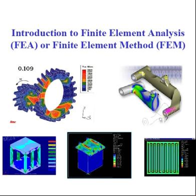
Fea Theory 1n5u3
November 2019 59
Fea Theory 1n5u3
November 2022 0
Fea Report.pdf 3a475e
November 2021 0
Fea Procedure 4y3733
December 2019 63
Catia Fea 2y2y5q
August 2020 0More Documents from "Samira Gh" m1t1h
Tank Fea 334v5f
April 2020 29
4p345f
April 2020 52
Metodologias De Desarrollo Software 6a3r3q
September 2020 0
La Medicina En La America Precolombina.docx 2r2s2p
November 2019 59
Mercy And Justice In The Merchant Of Venice Essay 394q6p
October 2021 0